Page 336 - Linear Models for the Prediction of Animal Breeding Values 3rd Edition

1. For each animal i with missing observations:
[k]
ˆ [k]
ˆ
(1a) calculate y ˆ [k] , given b and a using Eqn e.1;
im
*
(1b) transform y to the canonical scale: yˆ = Qyˆ .
ˆ
i i i
ˆ
2. Solve the MME to obtain solutions in the canonical scale: b* [k+1] and aˆ* [k+1] .
−1
ˆ [k+1]
3. Back-transform using Q to obtain b and â [k+1] .
4. If convergence is not achieved, go to 1.
Ducrocq and Besbes (1993) showed that it is possible to update y (step 1) without
back-transforming to the original scale (step 3) in each round of iteration. Suppose
that the vector of observations for animal i with missing records, y , is ordered such
i
that observed records precede missing values: y′ = [y′ , y′ ], and rows and columns
i iv im
−1
−1
of R, Q and Q are ordered accordingly. Partition Q as (Q | Q ) and Q as:
v m
⎡ Q ⎤
v
Q −1 = ⎢ ⎥
⎣ ⎢ Q ⎥ ⎦
m
*
ˆ
then from Eqn e.1, the equation for Qy or yˆ (see 1b) is:
i i
y = Q y + Q [x′ b + aˆ + R R (y − x′ b − a )] (e.2)
ˆ [k]
−1
ˆ [k]
[k]
ˆ
*
ˆ
[k]
i v iv m im im mv vv iv iv iv
However:
v * ˆ ⎤
⎡ b ˆ ⎤ − 1 ˆ * ⎡ Qb
iv
⎢ ⎥ = Q b = ⎢ ⎥
m * ˆ
⎣ b ˆ im⎦ ⎢ ⎣ Qb ⎥ ⎦
ˆ
and a similar expression exists for â. Substituting these values for b and aˆ in
Eqn e.2:
−1
ˆ *[k]
−1
v
m
ˆ
y* = (Q + Q R R )y + (Q Q − Q R R Q )(x′ b + a ˆ *[k] )
i v m mv vv iv m m mv vv i
ˆ *[k]
= Q y + Q (x ′b + ˆa *[k] ) (e.3)
1 iv 2 i
v
m
−1
−1
with Q = Q + Q R R and Q = (Q Q − Q R R Q )
1 v m mv vv 2 m m mv vv
*
ˆ
Thus for an animal with missing records, y in Eqn e.3 is the updated vector of
i
observation transformed to canonical scale (steps 1a and 1b above) and this is calcu-
lated directly without back-transformation to the original scale (step 3). The matrices
Q and Q in Eqn e.3 depend on the missing pattern and if there are n missing pat-
1 2
terns, n such matrices of each type must be set up initially and stored for use at each
iteration.
E.2.1 Illustration
Using the same genetic parameters and data as for Example 5.3, the above methodol-
ogy is employed to estimate sex effects and predict breeding values for pre-weaning
weight and post-weaning gain iterating on the data (see Section 17.4).
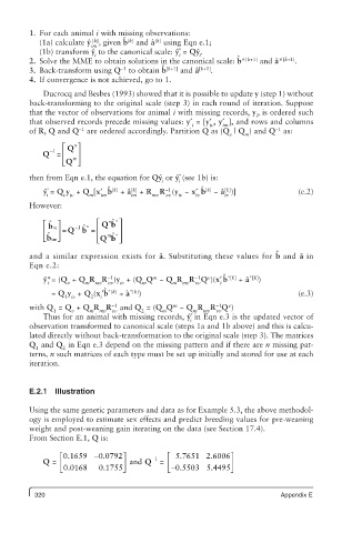
From Section E.1, Q is:
é 0.1659 - 0.0792ù é 5.7651 2.6006ù
Q = ê ú and Q - 1 = ê ú
ë 0.0168 0.1755 û ë - -0.5503 5.4495 û
320 Appendix E