Page 340 - Linear Models for the Prediction of Animal Breeding Values 3rd Edition

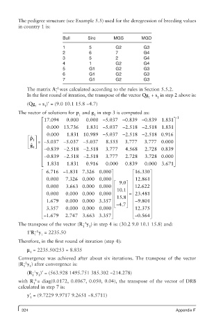
The pedigree structure (see Example 5.5) used for the deregression of breeding values
in country 1 is:
Bull Sire MGS MGD

1 5 G2 G3
2 6 7 G4
3 5 2 G4
4 1 G2 G4
5 G1 G2 G3
6 G1 G2 G3
7 G1 G2 G3

The matrix A was calculated according to the rules in Section 5.5.2.
−1
1
In the first round of iteration, the transpose of the vector Qg + s in step 2 above is:
1 1
(Qg + s )′ = (9.0 10.1 15.8 −4.7)
1 1
The vector of solutions for p and g in step 3 is computed as:
1 1
é 17.094 0.000 0.000 - 5.037 - 0.839 - 0.839 1.831ù -1
ê 1.831 - - 2.518 - ú
0
ê 0.000 13.736 5.037 2.518 1.831 ú
ê 0.000 1.831 10.989 - 5.037 - -2.518 -2.518 0.916ú
ˆ p é 1 ù ê ê ú
= -5.037
ê ú ê -5.037 -5.037 8.555 3.777 3.777 0.000 ú
ë ˆ g 1û ê - 2.518 - ú
ê -0..839 2.518 3.777 4.568 2.728 0.839 ú
ê - 0.839 - 2.518 - 2.518 3.7777 2.728 3.728 0.000 ú
ê ú
ë 1.831 1.831 0.916 0.000 0.839 0.000 3.671 û
é é 6.716 - 1.831 7.326 0.000ù é 16.330ù
0
ê ú ê ú
ê 0.000 7.3326 0.000 0.000 ú é 9.0 ù ê 12.861 ú
ê 0.000 3.663 0.000 0.000ú ê ú ê 12.622ú
ê ú 10.1 ú ê ú
ê
ê 0.000 0.000 0.000 0.000 ú ú = 23.481 ú
ê
ê 1.679 0.000 0.000 3.357 ê ê15.8 ú ê - 9.801 ú
ú
9
ê ú - 4.7 û ê ú
ë
ê 3.357 0.000 0.000 0.000 ú ê 12.375 ú ú
ê ú ê ú
ë - 1.679 2.747 3.663 3.357 û ë - 0.564 û
−1
The transpose of the vector (R y ) in step 4 is: (30.2 9.0 10.1 15.8) and:
1 1
1′R y = 2235.50
−1
1 1
Therefore, in the first round of iteration (step 4):
m = 2235.50/253 = 8.835
1
Convergence was achieved after about six iterations. The transpose of the vector
(R y ) after convergence is:
−1
1 1
−1
(R y )′ = (563.928 1495.751 385.302 −214.278)
1 1
−1
with R = diag(0.0172, 0.0067, 0.050, 0.04), the transpose of the vector of DRB
1
calculated in step 7 is:
y′ = (9.7229 9.9717 9.2651 −8.5711)
1
324 Appendix F