Page 65 - Financial Statement Analysis

sub79433_ch01.qxd 4/7/08 11:21 AM Page 42

42 Financial Statement Analysis

the discounted expected future free cash flows using the weighted average cost of capital.
(Note, the value of equity equals the value of the entire firm less the value of debt.)
The residual income model computes value using accounting variables. It defines
equity value at time t as the sum of current book value and the present value of all future
expected residual income:

E(RI t 1 ) E(RI t 2 ) E(RI t 3 )
V t BV t
(1 k) 1 (1 k) 2 (1 k) 3
where BV is book value at the end of period t, RI t n is residual income in period t n,
t
and k is cost of capital. Residual income at time t is defined as comprehensive net
income minus a charge on beginning book value, that is, RI NI (k BV t 1 ).
t
t
While both of these models overcome some problems in using dividends, they still
are defined in terms of an infinite horizon. To derive value using a finite horizon (say,
5 or 10 years), we must replace the present value of future dividends beyond a particu-
lar future date by an estimate of continuing value (also called terminal value).
Unlike forecasts of payoffs for the finite period that often are derived using detailed
prospective analysis, a forecast of continuing value is usually based on simplifying
assumptions for growth in payoffs. While forecasting continuing value often is a source
of much error, its estimation is required in equity valuation.
Note that all three models—dividend discount, free cash flow to equity, and residual
income—are identical and exact in an infinite horizon. Therefore, choosing a valuation
model is based on practical considerations in a finite horizon setting. Moreover, an im-
portant criterion is to choose a valuation model least dependent on continuing value.
While the free cash flow to equity and dividend discount models work well under cer-
tain circumstances in finite horizons, the residual income model usually outperforms
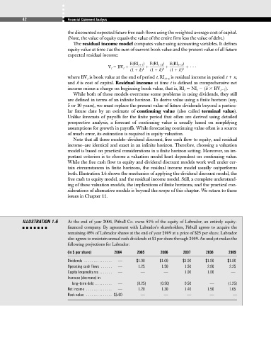
both. Illustration 1.6 shows the mechanics of applying the dividend discount model, the
free cash to equity model, and the residual income model. Still, a complete understand-
ing of these valuation models, the implications of finite horizons, and the practical con-
siderations of alternative models is beyond the scope of this chapter. We return to these
issues in Chapter 11.

ILLUSTRATION 1.6 At the end of year 2004, Pitbull Co. owns 51% of the equity of Labrador, an entirely equity-
financed company. By agreement with Labrador’s shareholders, Pitbull agrees to acquire the
remaining 49% of Labrador shares at the end of year 2009 at a price of $25 per share. Labrador
also agrees to maintain annual cash dividends at $1 per share through 2009. An analyst makes the
following projections for Labrador:
(in $ per share) 2004 2005 2006 2007 2008 2009
Dividends . . . . . . . . . . . . . . . — $1.00 $1.00 $1.00 $1.00 $1.00
Operating cash flows . . . . . . — 1.25 1.50 1.50 2.00 2.25
Capital expenditures . . . . . . . — — — 1.00 1.00 —
Increase (decrease) in
long-term debt . . . . . . . . . — (0.25) (0.50) 0.50 — (1.25)
Net income . . . . . . . . . . . . . . — 1.20 1.30 1.40 1.50 1.65
Book value . . . . . . . . . . . . . . $5.00 — — — — —