Page 417 - Microeconomics, Fourth Edition

c10competitive markets applications.qxd 7/15/10 4:58 PM Page 391

10.1 THE INVISIBLE HAND, EXCISE TAXES, AND SUBSIDIES 391

V
$20
S + $6

Price (dollars per unit) $12 E M J R S

$10
$8
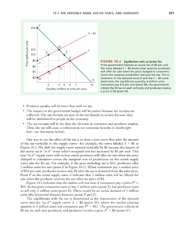
FIGURE 10.2
Equilibrium with an Excise Tax
If the government imposes an excise tax of $6 per unit,
A
$6
the curve labeled S $6 shows what quantity producers
N
$4 will offer for sale when the price charged to consumers
covers the marginal production cost plus the tax. The in-
F
$2 tersection of the demand curve D and the S $6 curve
determines the equilibrium quantity, 4 million units.
W
D
2 4 5 6 7 10 Consumers pay $12 per unit (point M), the government
Quantity (millions of units per year) collects the $6 tax on each unit sold, and producers receive
a price of $6 (point N).
• Producer surplus will be lower than with no tax.
• The impact on the government budget will be positive because tax receipts are
collected. The tax receipts are part of the net benefit to society because they
will be distributed to people in the economy.
• The tax receipts will be less than the decrease in consumer and producer surplus.
Thus, the tax will cause a reduction in net economic benefits (a deadweight
loss—see discussion below).

One way to see the effect of the tax is to draw a new curve that adds the amount
of the tax vertically to the supply curve—for example, the curve labeled S $6 in
Figure 10.2. We shift the supply curve upward vertically by $6 because the impact of
the excise tax is “as if” every seller’s marginal cost has increased by $6 per unit. This
new “as if” supply curve tells us how much producers will offer for sale when the price
charged to consumers covers the marginal cost of production on the actual supply
curve plus the $6 tax. For example, if the price including tax is $10, producers offer
2 million units for sale (point E in Figure 10.2). When consumers pay a market price
of $10 per unit, producers receive only $4 after the tax is deducted from the sales price.
Point F on the actual supply curve S indicates that 2 million units will be offered for
sale when the producer receives the net after-tax price of $4.
d
Figure 10.2 indicates that the market will not clear if consumers pay a price P
$10. At that price consumers want to buy 5 million units (point J), but producers want
to sell only 2 million units (point E). There would be an excess demand of 3 million
units (the horizontal distance between points E and J ).
The equilibrium with the tax is determined at the intersection of the demand
curve and the “as if” supply curve, S $6 (point M), where the market-clearing
d
quantity is 4 million units and consumers pay P $12. The government collects its
s
$6 tax on each unit produced, and producers receive a price P $6 (point N ).