Page 422 - Microeconomics, Fourth Edition

c10competitive markets applications.qxd 7/15/10 4:58 PM Page 396

396 CHAPTER 10 COMPETITIVE MARKETS: APPLICATIONS

APPLICA TION 10.1
Gallons and Dollars: Gasoline Taxes In this application we assume that the demand
and supply curves are both linear and that the elastic-
ities are correct at the equilibrium with the excise tax
In 2009, about 140 billion gallons of gasoline were
of $0.40 per gallon. Let’s begin by determining the
purchased annually in the United States. Consumer
equation of the demand curve, which must pass
prices for gasoline fluctuate a great deal over time
through point R in Figure 10.5, where the price is
and vary by region, but the average price consumers
d
paid at the pump (P ) was about $2.65 per gallon. $2.65 and the quantity (measured in billions of gallons)
is 140. If the demand curve is linear, it has the form:
Taxes on gasoline are often imposed at the federal
level, but also by state and local governments. Thus, Q a bP d (10.2)
d
the taxes vary by region. In 2009 the federal tax was
Using the data, let us find the constants a and
18.4 cents per gallon, and the average state and local
b in equation (10.2). By definition, the own-price
tax was just under 22 cents per gallon. Thus, the total
d
d
elasticity of demand is Q ,P (¢Q/¢P)(P /Q ). In the
d
tax per gallon averaged about 40 cents per gallon.
linear demand curve, ¢Q/¢P b. Thus, 0.5
In a “back-of-the-envelope” exercise, let’s assume
d
b(2.65/140), or b 26.42. Now we know that Q
that the tax on gasoline (T) was $0.40 per gallon. This d
s
means that the price producers received (P ) was a 26.42P . We can calculate a by using the price and
quantity data at point R. Thus, 140 a 26.42(2.65),
about $2.25 per gallon. Studies have shown that in
so a 210. The equation of the demand curve is
the intermediate run (say, two to five years) the own-
d
d
Q 210 26.43P .
price elasticities of demand and supply are about
The equation of a linear supply curve is:
Q d ,P 0.5 and Q s ,P 0.4. Using the information
about the current equilibrium, let’s examine two Q e fP s (10.3)
s
questions:
Now let us find e and f. By definition, the own-
1. What quantities and prices would we anticipate price elasticity of supply is Q ,P (¢Q/¢P)(P /Q ). In
s
s
s
if the taxes were removed? equation (10.3), ¢Q/¢P f. Thus, at point W in
2. By how much do gasoline tax revenues rise for Figure 10.5, 0.4 f(2.25/140), or f 24.89. Therefore,
s
s
each one-cent increase in the gasoline tax? Q e 24.89P .
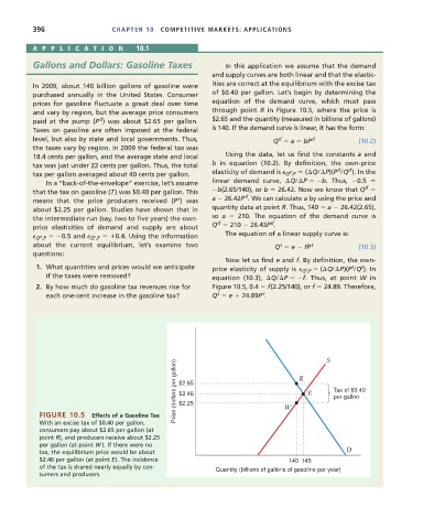
Price (dollars per gallon) $2.65 R E S Tax of $0.40
$2.46
per gallon
FIGURE 10.5 Effects of a Gasoline Tax $2.25 W
With an excise tax of $0.40 per gallon,
consumers pay about $2.65 per gallon (at
point R), and producers receive about $2.25
per gallon (at point W ). If there were no
tax, the equilibrium price would be about D
$2.46 per gallon (at point E). The incidence 140 145
of the tax is shared nearly equally by con- Quantity (billions of gallons of gasoline per year)
sumers and producers.