Page 427 - Microeconomics, Fourth Edition

c10competitive markets applications.qxd 7/15/10 4:58 PM Page 401

10.2 PRICE CEILINGS AND FLOORS 401
• Producer surplus will be lower than with no price ceiling.
• Some (but not all) of the lost producer surplus will be transferred to consumers.
• Because there is excess demand with a price ceiling, the size of the consumer sur-
plus will depend on which of the consumers who want the good are able to pur-
chase it. Consumer surplus may either increase or decrease with a price ceiling.
• There will be a deadweight loss.

Let’s examine the effects of a price ceiling in the form of rent controls. For
decades rent controls have been in force in many cities around the world. Rent con-
trols are legally imposed ceilings on the rents that landlords may charge their tenants.
They often originated as temporary ceilings imposed in the inflationary time of war,
as was the case in London and Paris during World War I, in New York during World
War II, and in Boston and several nearby suburbs during the Vietnam conflict in the
late 1960s and early 1970s.
In 1971 President Richard Nixon imposed wage and price controls throughout
the United States, freezing all rents. After the federal controls expired, many city gov-
ernments continued to place ceilings on rents. In 1997 William Tucker noted,
“During the 1970s it appeared that rent control might be the wave of the future. . . .
By the mid-1980s, more than 200 separate municipalities nationwide, encompassing
about 20 percent of the nation’s population, were living under rent control. However,
this proved to be the high tide of the movement. As inflationary pressures eased, the
agitation for rent control subsided.” 5
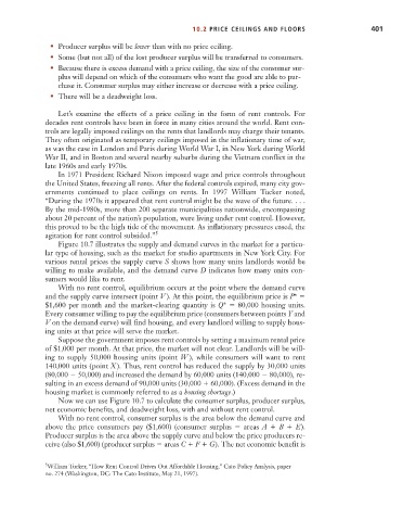
Figure 10.7 illustrates the supply and demand curves in the market for a particu-
lar type of housing, such as the market for studio apartments in New York City. For
various rental prices the supply curve S shows how many units landlords would be
willing to make available, and the demand curve D indicates how many units con-
sumers would like to rent.
With no rent control, equilibrium occurs at the point where the demand curve
and the supply curve intersect (point V ). At this point, the equilibrium price is P*
$1,600 per month and the market-clearing quantity is Q* 80,000 housing units.
Every consumer willing to pay the equilibrium price (consumers between points Y and
V on the demand curve) will find housing, and every landlord willing to supply hous-
ing units at that price will serve the market.
Suppose the government imposes rent controls by setting a maximum rental price
of $1,000 per month. At that price, the market will not clear. Landlords will be will-
ing to supply 50,000 housing units (point W ), while consumers will want to rent
140,000 units (point X ). Thus, rent control has reduced the supply by 30,000 units
(80,000 50,000) and increased the demand by 60,000 units (140,000 80,000), re-
sulting in an excess demand of 90,000 units (30,000 60,000). (Excess demand in the
housing market is commonly referred to as a housing shortage.)
Now we can use Figure 10.7 to calculate the consumer surplus, producer surplus,
net economic benefits, and deadweight loss, with and without rent control.
With no rent control, consumer surplus is the area below the demand curve and
above the price consumers pay ($1,600) (consumer surplus areas A B E).
Producer surplus is the area above the supply curve and below the price producers re-
ceive (also $1,600) (producer surplus areas C F G). The net economic benefit is

5 William Tucker, “How Rent Control Drives Out Affordable Housing,” Cato Policy Analysis, paper
no. 274 (Washington, DC: The Cato Institute, May 21, 1997).