Page 425 - Microeconomics, Fourth Edition

c10competitive markets applications.qxd 7/15/10 4:58 PM Page 399

10.1 THE INVISIBLE HAND, EXCISE TAXES, AND SUBSIDIES 399
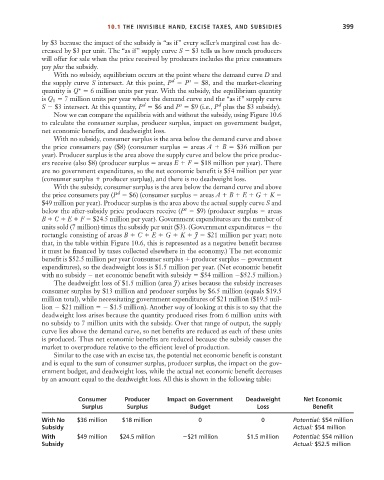
by $3 because the impact of the subsidy is “as if” every seller’s marginal cost has de-
creased by $3 per unit. The “as if” supply curve S $3 tells us how much producers
will offer for sale when the price received by producers includes the price consumers
pay plus the subsidy.
With no subsidy, equilibrium occurs at the point where the demand curve D and
d
s
the supply curve S intersect. At this point, P P $8, and the market-clearing
quantity is Q* 6 million units per year. With the subsidy, the equilibrium quantity
is Q 7 million units per year where the demand curve and the “as if” supply curve
1
d
d
s
S $3 intersect. At this quantity, P $6 and P $9 (i.e., P plus the $3 subsidy).
Now we can compare the equilibria with and without the subsidy, using Figure 10.6
to calculate the consumer surplus, producer surplus, impact on government budget,
net economic benefits, and deadweight loss.
With no subsidy, consumer surplus is the area below the demand curve and above
the price consumers pay ($8) (consumer surplus areas A B $36 million per
year). Producer surplus is the area above the supply curve and below the price produc-
ers receive (also $8) (producer surplus areas E F $18 million per year). There
are no government expenditures, so the net economic benefit is $54 million per year
(consumer surplus producer surplus), and there is no deadweight loss.
With the subsidy, consumer surplus is the area below the demand curve and above
d
the price consumers pay (P $6) (consumer surplus areas A B E G K
$49 million per year). Producer surplus is the area above the actual supply curve S and
s
below the after-subsidy price producers receive (P $9) (producer surplus areas
B C E F $24.5 million per year). Government expenditures are the number of
units sold (7 million) times the subsidy per unit ($3). (Government expenditures the
rectangle consisting of areas B C E G K J $21 million per year; note
that, in the table within Figure 10.6, this is represented as a negative benefit because
it must be financed by taxes collected elsewhere in the economy.) The net economic
benefit is $52.5 million per year (consumer surplus producer surplus government
expenditures), so the deadweight loss is $1.5 million per year. (Net economic benefit
with no subsidy net economic benefit with subsidy $54 million $52.5 million.)
The deadweight loss of $1.5 million (area J) arises because the subsidy increases
consumer surplus by $13 million and producer surplus by $6.5 million (equals $19.5
million total), while necessitating government expenditures of $21 million ($19.5 mil-
lion $21 million $1.5 million). Another way of looking at this is to say that the
deadweight loss arises because the quantity produced rises from 6 million units with
no subsidy to 7 million units with the subsidy. Over that range of output, the supply
curve lies above the demand curve, so net benefits are reduced as each of these units
is produced. Thus net economic benefits are reduced because the subsidy causes the
market to overproduce relative to the efficient level of production.
Similar to the case with an excise tax, the potential net economic benefit is constant
and is equal to the sum of consumer surplus, producer surplus, the impact on the gov-
ernment budget, and deadweight loss, while the actual net economic benefit decreases
by an amount equal to the deadweight loss. All this is shown in the following table:

Consumer Producer Impact on Government Deadweight Net Economic
Surplus Surplus Budget Loss Benefit
With No $36 million $18 million 0 0 Potential: $54 million
Subsidy Actual: $54 million
With $49 million $24.5 million $21 million $1.5 million Potential: $54 million
Subsidy Actual: $52.5 million