Page 423 - Microeconomics, Fourth Edition

c10competitive markets applications.qxd 7/15/10 4:58 PM Page 397

10.1 THE INVISIBLE HAND, EXCISE TAXES, AND SUBSIDIES 397

We can calculate e by using the price and quan- producers. This is not surprising because the elastici-
tity data at point W. Thus, 140 e 24.89(2.25), so ties of supply and demand are about the same.
s
e 84. Thus, the equation of the supply curve is Q With the tax, consumers pay $2.65 instead of $2.46
s
84 24.89P . per gallon, while producers receive $2.25 instead
The supply and demand curves are drawn in of $2.46.
Figure 10.5. If there were no taxes, the equilibrium We can repeat Learning-By-Doing Exercise 10.1
would be at point E, where the equilibrium price to find how different levels of the gasoline tax will
d
s
P* P P (there is no tax wedge). Since the mar- affect the quantity sold, the prices paid by consumers
d
s
ket clears (Q Q ), we know that 210 26.43P* and received by producers, and the revenues from
84 24.89P*, so the equilibrium price is P* 2.46. With gasoline taxes. The following table shows the results
no tax, about 145 billion gallons of gas would be sold. of this exercise (the calculations are not shown, but
The incidence of the current tax (T $0.40 per you should be able to do them yourself) for taxes
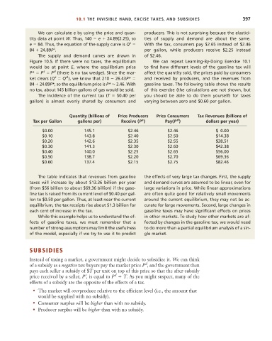
gallon) is almost evenly shared by consumers and varying between zero and $0.60 per gallon.
Quantity (billions of Price Producers Price Consumers Tax Revenues (billions of
s
d
Tax per Gallon gallons per) Receive (P ) Pay(P ) dollars per year)
$0.00 145.1 $2.46 $2.46 $ 0.00
$0.10 143.8 $2.40 $2.50 $14.38
$0.20 142.6 $2.35 $2.55 $28.51
$0.30 141.3 $2.30 $2.60 $42.38
$0.40 140.0 $2.25 $2.65 $56.00
$0.50 138.7 $2.20 $2.70 $69.36
$0.60 137.4 $2.15 $2.75 $82.46

The table indicates that revenues from gasoline the effects of very large tax changes. First, the supply
taxes will increase by about $13.36 billion per year and demand curves are assumed to be linear, even for
(from $56 billion to about $69.36 billion) if the gaso- large variations in price. While linear approximations
line tax is raised from its current level of $0.40 per gal- are often quite good for relatively small movements
lon to $0.50 per gallon. Thus, at least near the current around the current equilibrium, they may not be ac-
equilibrium, the tax receipts rise about $1.3 billion for curate for large movements. Second, large changes in
each cent of increase in the tax. gasoline taxes may have significant effects on prices
While this example helps us to understand the ef- in other markets. To study how other markets are af-
fects of gasoline taxes, we must remember that a fected by changes in the gasoline tax, we would need
number of strong assumptions may limit the usefulness to do more than a partial equilibrium analysis of a sin-
of the model, especially if we try to use it to predict gle market.

SUBSIDIES

Instead of taxing a market, a government might decide to subsidize it. We can think
d
of a subsidy as a negative tax: buyers pay the market price P , and the government then
pays each seller a subsidy of $T per unit on top of this price so that the after-subsidy
s
d
price received by a seller, P , is equal to P T. As you might suspect, many of the
effects of a subsidy are the opposite of the effects of a tax.
• The market will overproduce relative to the efficient level (i.e., the amount that
would be supplied with no subsidy).
• Consumer surplus will be higher than with no subsidy.
• Producer surplus will be higher than with no subsidy.