Page 418 - Microeconomics, Fourth Edition

c10competitive markets applications.qxd 7/15/10 4:58 PM Page 392

392 CHAPTER 10 COMPETITIVE MARKETS: APPLICATIONS

$20 Area Size (dollars/year)
$16 million
A
S + $6 8 million
B
8 million
C 4 million
Price (dollars per unit) P = $12 B C E S G 8 million
E
2 million
F
A
8 million
d
H
$8
G
P = $6
s
H F
$2
D
4 6 10
Quantity (millions of units per year)

With No Tax With Tax Impact of Tax
C onsumer surplus A + B + C + E A ($16 million) –B – C – E
($36 million) ( –$20 million)
Producer surplus F + G + H ($18 million) H ($8 million) –F – G ( –$10 million)
Government receipts from tax zero B + C + G ($24 million) B + C + G ($24 million)

Net benefits (consumer surplus + A + B + C + E + A + B + C + G + H –E – F
producer surplus + g ov ernment F + G + H ($48 million) ( –$6 million)
re c eipts) ($54 million)

Deadweight loss zero E + F ($6 million) E + F ($6 million)

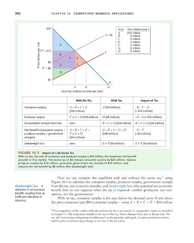
FIGURE 10.3 Impact of a $6 Excise Tax
With no tax, the sum of consumer and producer surplus is $54 million, the maximum net benefit
possible in this market. The excise tax of $6 reduces consumer surplus by $20 million, reduces
producer surplus by $10 million, generates government tax receipts of $24 million, and
reduces the net benefit by $6 million (the deadweight loss).

3
Now we can compare the equilibria with and without the excise tax, using
Figure 10.3 to calculate the consumer surplus, producer surplus, government receipts
deadweight loss A from the tax, net economic benefits, and deadweight loss (the potential net economic
reduction in net economic benefit that no one captures when the tax is imposed—neither producers, nor con-
benefits resulting from an sumers, nor the government).
inefficient allocation of With no tax, consumer surplus is the area below the demand curve D and above
resources.
the price consumers pay ($8) (consumer surplus areas A B C E $36 million
3 The comparison of the market with and without the tax is an exercise in comparative statics, as described
in Chapter 1. The exogenous variable is the size of the tax, which changes from zero to $6 per unit. We
can ask how various endogenous variables (such as the quantity exchanged, the price producers receive,
and the price consumers pay) change as the size of the tax varies.