Page 474 - Microeconomics, Fourth Edition

c11monopolyandmonopsony.qxd 7/14/10 7:58 PM Page 448

448 CHAPTER 11 MONOPOLY AND MONOPSONY

$12 A MC
Price (dollars per ounce) $8 B

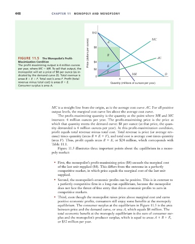
FIGURE 11.5 The Monopolist’s Profit- AC
Maximization Condition $4
The profit-maximizing output is 4 million ounces E
per year, where MC MR. To sell that output, the $2
monopolist will set a price of $8 per ounce (as in- F MR D
dicated by the demand curve D). Total revenue is 0
areas B E F. Total cost is area F. Profit (total 4
revenue minus total cost) is areas B E. Quantity (millions of ounces per year)
Consumer surplus is area A.

MC is a straight line from the origin, as is the average cost curve AC. For all positive
output levels, the marginal cost curve lies above the average cost curve.
The profit-maximizing quantity is the quantity at the point where MR and MC
intersect: 4 million ounces per year. The profit-maximizing price is the price at
which that quantity meets the demand curve: $8 per ounce (at that price, the quan-
tity demanded is 4 million ounces per year). At this profit-maximization condition,
profit equals total revenue minus total cost. Total revenue is price (or average rev-
enue) times quantity (areas B E F), and total cost is average cost times quantity
(area F). Thus, profit equals areas B E, or $24 million, which corresponds with
Table 11.1.
Figure 11.5 illustrates three important points about the equilibrium in a mono-
poly market:

• First, the monopolist’s profit-maximizing price ($8) exceeds the marginal cost
of the last unit supplied ($4). This differs from the outcome in a perfectly
competitive market, in which price equals the marginal cost of the last unit
supplied.
• Second, the monopolist’s economic profits can be positive. This is in contrast to
a perfectly competitive firm in a long-run equilibrium, because the monopolist
does not face the threat of free entry that drives economic profits to zero in
competitive markets.
• Third, even though the monopolist raises price above marginal cost and earns
positive economic profits, consumers still enjoy some benefits at the monopoly
equilibrium. The consumer surplus at the equilibrium in Figure 11.5 is the area
between price and the demand curve, or area A, which equals $8 million. The
total economic benefit at the monopoly equilibrium is the sum of consumer sur-
plus and the monopolist’s producer surplus, which is equal to areas A B E,
or $32 million per year.