Page 478 - Microeconomics, Fourth Edition

c11monopolyandmonopsony.qxd 7/14/10 7:58 PM Page 452

452 CHAPTER 11 MONOPOLY AND MONOPSONY
marginal revenue (and therefore between total revenue and price), as shown in the fol-
lowing table:

Relationship between
Region of Demand Curve Marginal Revenue and Q,P Total Revenue and Price

Elastic ( q Q,P 1) MR 0 The monopolist can in-
[because 1 (1/ Q,P ) 0] crease total revenue by
decreasing price (and
thereby increasing quan-
tity) by a small amount.
Unitary elastic ( Q,P 1) MR 0 The monopolist’s total
[because 1 (1/ Q,P ) 0] revenue will not change
when price (or quantity)
is changed by a small
amount.
Inelastic ( 1 Q,P 0) MR 0 The monopolist can in-
[because 1 (1/ Q,P ) 0] crease total revenue by
increasing price (and
thereby decreasing quan-
tity) by a small amount.

This table reflects our discussion in Chapter 2 of how a firm’s total revenue re-
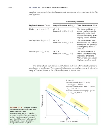
sponds to a price change. The relationship between marginal revenue and price elas-
ticity of demand shown in the table is illustrated in Figure 11.8.

P = a – bQ
Demand is elastic when Q < a/(2b):
–∞ < ε Q,P < –1, MR > 0
Demand is unitary elastic when Q = a/(2b):
ε = –1, MR = 0
Q,P
a Elastic region Demand is inelastic when a/(2b) < Q < a/b:
–1 < ε Q,P < 0, MR < 0
P (dollars per unit)

FIGURE 11.8 Marginal Revenue MR D
Inelastic region
and Price Elasticity of Demand for a
Linear Demand Curve
Where demand is elastic, marginal
revenue is positive. Where demand is
unitary elastic, marginal revenue is 0 a a
zero (i.e., MR crosses the horizontal 2b b
axis). Where demand is inelastic, Quantity Q (units per year)
marginal revenue is negative.