Page 72 - Microeconomics, Fourth Edition

c02demandandsupplyanalysis.qxd 6/14/10 1:39 PM Page 46

46 CHAPTER 2 DEMAND AND SUPPLY ANALYSIS
curve by taking the equation for the demand curve and solving it for P in terms of Q.
The inverse demand curve for the linear demand curve is given by

a 1
P Q
b b

choke price The price The term a b is called the choke price. This is the price at which the quantity
at which quantity demanded falls to 0. 10
demanded falls to 0. Using equation (2.3), we see that the price elasticity of demand for the linear
demand curve in Figure 2.16 is given by the formula

¢Q P P
Q, P b (2.4)
¢P Q Q
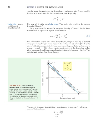
This formula tells us that for a linear demand curve, the price elasticity of demand
varies as we move along the curve. Between the choke price a b (where Q 0) and a
price of a 2b at the midpoint M of the demand curve, the price elasticity of demand is
between q and 1. This is known as the elastic region of the demand curve. For
prices between a 2b and 0, the price elasticity of demand is between 1 and 0. This
is the inelastic region of the demand curve.

a ε Q,P = –∞ Q = a – bP
b
ε or
a Q
P = –
Q,P
b b
Elastic region
Price (dollars per unit) 2b M ε Q,P = –1
a
between –∞ and –1

ε

FIGURE 2.16 Price Elasticity of Q,P Inelastic region
Demand along a Linear Demand Curve between –1 and 0
In the region to the northwest of the mid- D
point M, demand is elastic, with the price ε = 0
elasticity of demand between minus infinity Q,P
and 1. In the region to the southeast of 0 a a
the midpoint M, demand is inelastic, with 2
the price elasticity of demand between 1 Quantity (units per year)
and 0.

10 You can verify that quantity demanded falls to 0 at the choke price by substituting P a b into the
equation of the demand curve:
a
Q a b a b
b
a a
0