Page 768 - Microeconomics, Fourth Edition

BMappAMathematicalAppendix.qxd 8/17/10 1:10 AM Page 742

742 MATHEMATICAL APPENDIX

that maximize a dependent variable (p in the example). To 0p
Q 1 8 4Q 2 (A.11)
do so, we need to understand how a change in each of the 0Q 2
independent variables affects the dependent variable, hold- Equation (A.11) measures the marginal profit (some-
ing constant the levels of all other independent variables. times called marginal profitability) of Q 2 . This marginal
Consider point B in the graph, where Q 1 4 , Q 2 2 , profit is the rate of change of profit (and the slope of the
and p 36 . As the graph shows, this is not the combination profit hill) as we vary Q 2 , but hold Q 1 constant.
of outputs that maximizes profit. We illustrate what this partial derivative measures in
The firm might ask how an increase in Q 2 affects p, Figure A.8. At point B we have drawn a line tangent to the
holding constant the other independent variable Q 1 . To profit hill (line RS). Along RS we are holding Q 1 constant
find this information, we find the partial derivative of p (Q 1 4 ). We can find the slope of RS by evaluating the
with respect to Q 2 , denoted by 0p/0Q 2 . To obtain this partial
partial derivative 0p/0Q 2 Q 1 8 4Q 2 when Q 1 4
derivative, we take the derivative of equation (A.10), but and Q 2 2 . The value of the derivative is therefore
treat the level of Q 1 as a constant. When we do this, the first 0p/0Q 2 (4) 8 4(2) 4 . The slope of RS (and there-
two terms in equation (A.10) will be a constant because they fore the slope of the profit hill at B in the direction of increas-
depend only on Q 1 ; therefore the partial derivative of these ing Q 2 ) is 4.
terms with respect to Q 2 is zero. The partial derivative of To help you understand the meaning of a partial deriv-
the third term (Q 1 Q 2 ) with respect to Q 2 is just Q 1 . The par- ative, we have provided another view of the profit hill in
tial derivative of the last two terms [8Q 2 2(Q 2 ) 2 ] with Figure A.9. This graph shows a cross-sectional picture of
respect to Q 2 will be 8 4Q 2 . When we put all of this the profit hill, showing what the profit hill looks like when
information together, we learn that

S Slope of
40
E F tangent line
A EF = 0
B

30
R

Slope of
tangent line
Profit, π 20 RS = +4 Profit curve when Q = 4
1

10

0 1 2 3 4 5 6
Q
2
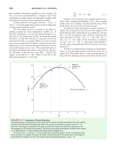
FIGURE A.9 Illustration of Partial Derivative
The graph shows a cross section of the profit hill in Figure A.8. We have drawn the cross section
to show what the profit hill looks like when we vary Q 2 , but hold Q 1 constant, with Q 1 4 .
Point B in this figure is therefore the same as point B in Figure A.8. We have also drawn the
line tangent to the profit hill at point B. The value of the partial derivative of profit with respect
to Q 2 (denoted by 0p/0Q 2 ) measures the slope of this tangent line.
At point A, Q 1 4 and Q 2 3 , the outputs that maximize profits. Point A is therefore the
same as point A in Figure A.8. Since we have reached the top of the profit curve, the slope of
the profit hill in Figure A.9 is 0. This means that the partial derivative 0p/0Q 2 0 .