Page 221 - Economics

CONFIRMING PAGES

PART THREE
192
Macroeconomic Models and Fiscal Policy
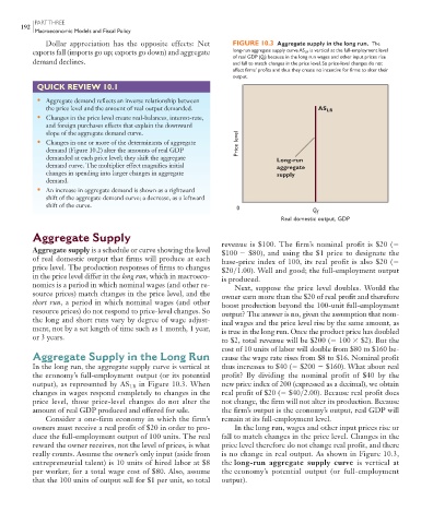
Dollar appreciation has the opposite effects: Net FIGURE 10.3 Aggregate supply in the long run. The
exports fall (imports go up; exports go down) and aggregate long-run aggregate supply curve AS LR is vertical at the full-employment level
of real GDP (Q f ) because in the long run wages and other input prices rise
demand declines. and fall to match changes in the price level. So price-level changes do not
affect firms’ profits and thus they create no incentive for firms to alter their
output.
QUICK REVIEW 10.1
• Aggregate demand reflects an inverse relationship between
the price level and the amount of real output demanded. AS LR
• Changes in the price level create real-balances, interest-rate,
and foreign purchases effects that explain the downward
slope of the aggregate demand curve.
• Changes in one or more of the determinants of aggregate Price level
demand (Figure 10.2) alter the amounts of real GDP
demanded at each price level; they shift the aggregate
Long-run
demand curve. The multiplier effect magnifies initial aggregate
changes in spending into larger changes in aggregate supply
demand.
• An increase in aggregate demand is shown as a rightward
shift of the aggregate demand curve; a decrease, as a leftward
shift of the curve.
0
Q f
Real domestic output, GDP
Aggregate Supply
revenue is $100. The firm’s nominal profit is $20 (
Aggregate supply is a schedule or curve showing the level $100 $80), and using the $1 price to designate the
of real domestic output that firms will produce at each base-price index of 100, its real profit is also $20 (
price level. The production responses of firms to changes $20 1.00). Well and good; the full-employment output
in the price level differ in the long run , which in macroeco- is produced.
nomics is a period in which nominal wages (and other re- Next, suppose the price level doubles. Would the
source prices) match changes in the price level, and the owner earn more than the $20 of real profit and therefore
short run , a period in which nominal wages (and other boost production beyond the 100-unit full-employment
resource prices) do not respond to price-level changes. So output? The answer is no, given the assumption that nom-
the long and short runs vary by degree of wage adjust- inal wages and the price level rise by the same amount, as
ment, not by a set length of time such as 1 month, 1 year, is true in the long run. Once the product price has doubled
or 3 years. to $2, total revenue will be $200 ( 100 $2). But the
cost of 10 units of labor will double from $80 to $160 be-
Aggregate Supply in the Long Run cause the wage rate rises from $8 to $16. Nominal profit
In the long run, the aggregate supply curve is vertical at thus increases to $40 ( $200 $160). What about real
the economy’s full-employment output (or its potential profit? By dividing the nominal profit of $40 by the
output), as represented by AS in Figure 10.3 . When new price index of 200 (expressed as a decimal), we obtain
LR
changes in wages respond completely to changes in the real profit of $20 ( $40 2.00). Because real profit does
price level, those price-level changes do not alter the not change, the firm will not alter its production. Because
amount of real GDP produced and offered for sale. the firm’s output is the economy’s output, real GDP will
Consider a one-firm economy in which the firm’s remain at its full-employment level.
owners must receive a real profit of $20 in order to pro- In the long run, wages and other input prices rise or
duce the full-employment output of 100 units. The real fall to match changes in the price level. Changes in the
reward the owner receives, not the level of prices, is what price level therefore do not change real profit, and there
really counts. Assume the owner’s only input (aside from is no change in real output. As shown in Figure 10.3 ,
entrepreneurial talent) is 10 units of hired labor at $8 the long-run aggregate supply curve is vertical at
per worker, for a total wage cost of $80. Also, assume the economy’s potential output (or full-employment
that the 100 units of output sell for $1 per unit, so total output).

8/21/06 4:51:08 PM
mcc26632_ch10_187-207.indd 192 8/21/06 4:51:08 PM
mcc26632_ch10_187-207.indd 192