Page 225 - Economics

CONFIRMING PAGES

PART THREE
196
Macroeconomic Models and Fiscal Policy
gasoline supply. This reduces the per-unit production cost In Figure 10.6 the equilibrium price level and level of
of making blended gasoline. To the extent that this and real output are 100 and $510 billion, respectively. To illus-
other subsidies are successful, the aggregate supply curve trate why, suppose the price level is 92 rather than 100. We
shifts rightward. see from the table that the lower price level will encourage
businesses to produce real output of $502 billion. This is
Government Regulation It is usually costly for shown by point a on the AS curve in the graph. But, as
businesses to comply with government regulations. More revealed by the table and point b on the aggregate demand
regulation therefore tends to increase per-unit production curve, buyers will want to purchase $514 billion of real
costs and shift the aggregate supply curve to the left. “Sup- output at price level 92. Competition among buyers to pur-
ply-side” proponents of deregulation of the economy have chase the lesser available real output of $502
argued forcefully that, by increasing efficiency and reduc- billion will eliminate the $12 billion ( $514
ing the paperwork associated with complex regulations, billion $502 billion) shortage and pull up
deregulation will reduce per-unit costs and shift the ag- the price level to 100.
gregate supply curve to the right. Other economists are As the table and graph show, the rise in
less certain. Deregulation that results in accounting ma- the price level from 92 to 100 encourages
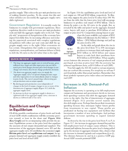
G 10.1
nipulations, monopolization, and business failures is likely producers to increase their real output from
Aggregate
to shift the AS curve to the left rather than to the right. demand–aggregate $502 billion to $510 billion and causes
supply buyers to scale back their purchases from
$514 billion to $510 billion. When equality
QUICK REVIEW 10.2
occurs between the amounts of real output produced and
• The long-run aggregate supply curve is vertical because, given purchased, as it does at price level 100, the economy has
sufficient time, wages and other input prices rise and fall to achieved equilibrium (here, at $510 billion of real GDP).
match price-level changes; because price-level changes do not Now let’s apply the AD-AS model to various situations
change real rewards, they do not change production decisions. that can confront the economy. For simplicity we will use P
• The short-run aggregate supply curve (or simply the and Q symbols, rather than actual numbers. Remember that
“aggregate supply curve”) is upward-sloping because wages these symbols represent price index values and amounts of
and other input prices do not immediately adjust to changes real GDP.
in price levels. The curve’s upward slope reflects rising per-
unit production costs as output expands.
• By altering per-unit production costs independent of Increases in AD: Demand-Pull
changes in the level of output, changes in one or more of the
determinants of aggregate supply (Figure 10.5) shift the Inflation
aggregate supply curve. Suppose the economy is operating at its full-employment
• An increase in short-run aggregate supply is shown as a output and businesses and government decide to increase
rightward shift of the aggregate supply curve; a decrease is their spending—actions that shift the aggregate demand
shown as a leftward shift of the curve. curve to the right. Our list of determinants of aggregate
demand ( Figure 10.2 ) provides several reasons why
this shift might occur. Perhaps firms boost their investment
Equilibrium and Changes spending because they anticipate higher future profits
in Equilibrium from investments in new capital. Those profits are
predicated on having new equipment and facilities that
Of all the possible combinations of price levels and levels incorporate a number of new technologies. And perhaps
of real GDP, which combination will the economy gravi- government increases spending to expand national
tate toward, at least in the short run? Figure 10.6 defense.
(Key Graph) and its accompanying table provide the an- As shown by the rise in the price level from P to P in
2
1
swer. Equilibrium occurs at the price level that equalizes Figure 10.7 , the increase in aggregate demand beyond the
the amounts of real output demanded and supplied. The full-employment level of output causes inflation. This is
intersection of the aggregate demand curve AD and the demand-pull inflation , because the price level is being pulled
aggregate supply curve AS establishes the economy’s equi- up by the increase in aggregate demand. Also, observe that
librium price level and equilibrium real output . So ag- the increase in demand expands real output from Q to Q .
1
f
gregate demand and aggregate supply jointly establish the The distance between Q and Q is a positive GDP gap.
1
f
price level and level of real GDP. Actual GDP exceeds potential GDP.

8/21/06 4:51:09 PM
mcc26632_ch10_187-207.indd 196
mcc26632_ch10_187-207.indd 196 8/21/06 4:51:09 PM