Page 664 - Economics

CONFIRMING PAGES

CHAPTER 29
573
Public Choice Theory and the Economics of Taxation
by differences in property-tax rates from locality to local- Division of Burden Since the government im-
ity. In general, property-tax rates are higher in poorer poses the tax on the sellers (suppliers), we can view the
areas, to make up for lower property values. tax as an addition to the marginal cost of the product.
Now sellers must get $2 more for each bottle to receive
Tax Incidence and Efficiency the same per-unit profit they were getting before the tax.
While sellers are willing to offer, for example, 5 million
Loss bottles of untaxed wine at $4 per bottle, they must now
Determining whether a particular tax is progressive, pro- receive $6 per bottle ( $4 $2 tax) to offer the same
portional, or regressive is complicated, because those on 5 million bottles. The tax shifts the supply curve upward
whom taxes are levied do not always pay the taxes. We (leftward) as shown in Figure 29.2 , where S t is the “after-
therefore need to try to locate the final resting place of a tax” supply curve.
tax, or the tax incidence . The tools of elasticity of supply The after-tax equilibrium price is $9 per bottle,
and demand will help. Let’s focus on a hypothetical excise whereas the before-tax equilibrium price was $8. So, in
tax levied on wine producers. Do the producers really pay this case, consumers pay half the $2 tax as a higher price;
this tax, or do they shift it to wine consumers? producers pay the other half in the form of a lower after-
tax per-unit revenue. That is, after remitting the $2 tax
Elasticity and Tax Incidence per unit to government, producers receive $7, or $1 less
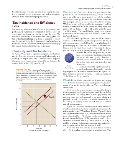
In Figure 29.2 , S and D represent the pretax market for a than the $8 before-tax price. So, in this
case, consumers and producers share the
certain domestic wine; the no-tax equilibrium price and burden of the tax equally: Producers
quantity are $8 per bottle and 15 million bottles. Suppose shift half the tax to consumers in the form
that government levies an excise tax of $2 per bottle at the of a higher price and bear the other half
winery. Who will actually pay this tax?
G 29.1 themselves.
Note also that the equilibrium quan-
Tax incidence
tity declines because of the tax levy and the
FIGURE 29.2 The incidence of an excise tax. An
excise tax of a specified amount, here $2 per unit, shifts the supply curve higher price that it imposes on consumers. In Figure 29.2
upward by the amount of the tax per unit: the vertical distance between that decline in quantity is from 15 million bottles to
S and S t . This results in a higher price (here $9) to consumers and a lower
after-tax price (here $7) to producers. Thus consumers and producers 12.5 million bottles per month.
share the burden of the tax in some proportion (here equally at
$1 per unit). Elasticities If the elasticities of demand and supply
P were different from those shown in Figure 29.2 , the inci-
dence of tax would also be different. Two generalizations
S t are relevant.
$14 With a specific supply, the more inelastic the demand
S
for the product, the larger is the portion of the tax shifted
12
to consumers. To verify this, sketch graphically the
Tax $2 extreme cases in which demand is perfectly elastic and
Price (per bottle) 8 is entirely on sellers; in the second, the tax is shifted
10
perfectly inelastic. In the first case, the incidence of the tax
entirely to consumers.

Figure 29.3 contrasts the more usual cases where de-
mand is either relatively elastic or relatively inelastic in the
6
relevant price range. With elastic demand ( Figure 29.3a ), a
small portion of the tax ( P P ) is shifted to consumers and
4 e 1
most of the tax ( P P ) is borne by the producers. With
1
a
D inelastic demand ( Figure 29.3b ), most of the tax ( P P ) is
2 i 1
shifted to consumers and only a small amount ( P P ) is
b
1
paid by producers. In both graphs the per-unit tax is repre-
0 5 10 15 20 25 Q sented by the vertical distance between S t and S.
Quantity Note also that the decline in equilibrium quantity
(millions of bottles per month) ( Q Q ) is smaller when demand is more inelastic. This
2
1

mcc26632_ch29_564-580.indd 573 9/10/06 9:41:04 PM
9/10/06 9:41:04 PM
mcc26632_ch29_564-580.indd 573