Page 666 - Economics

CONFIRMING PAGES

CHAPTER 29
575
Public Choice Theory and the Economics of Taxation
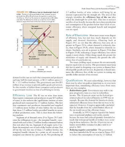
FIGURE 29.5 Effi ciency loss (or deadweight loss) of 2.5 million bottles of wine reduces well-being by an
a tax. The levy of a $2 tax per bottle of wine increases the price amount represented by the triangle abc. The area of this
per bottle from $8 to $9 and reduces the equilibrium quantity from
15 million to 12.5 million. Tax revenue to the government is $25 million triangle identifies the efficiency loss of the tax (also
(area efac ). The efficiency loss of the tax arises from the 2.5 million called the deadweight loss of the tax ). This loss is society’s
decline in output; the amount of that loss is shown as triangle abc. sacrifice of net benefit, because the tax reduces production
P and consumption of the product below their levels of eco-
Tax paid S t nomic efficiency, where marginal benefit and marginal
by consumers
$12 cost are equal.
S

10 Role of Elasticities Most taxes create some degree
f a Tax $2 of efficiency loss, but just how much depends on the
Price (per bottle) 8 6 e c b Figure 29.3 , we see that the efficiency loss area abc is
supply and demand elasticities. Glancing back at

greater in Figure 29.3a , where demand is relatively elas-
tic, than in Figure 29.3b , where demand is relatively in-
Efficiency
in Figure 29.4b , indicating a larger efficiency loss where
loss (or elastic. Similarly, area abc is greater in Figure 29.4a than
4
deadweight loss) supply is more elastic. Other things equal, the greater the
Tax paid elasticities of supply and demand, the greater the effi-
by producers D
2 ciency loss of a particular tax.
Two taxes yielding equal revenues do not necessarily
impose equal costs on society. The government must keep
0 5 10 15 20 25 Q this fact in mind in designing a tax system to finance ben-
Quantity eficial public goods and services. In general, it should min-
(millions of bottles per month) imize the efficiency loss of the tax system in raising any
specific dollar amount of tax revenue.
demand in this case are such that consumers and producers
each pay half this total amount, or $12.5 million apiece ( Qualifications We must acknowledge, however, that
$1 12.5 million bottles). The government uses this $25 there may be other tax goals as important as, or even more
million of tax revenue to provide public goods and services. important than, minimizing efficiency losses from taxes.
So this transfer of dollars from consumers and producers Here are two examples:
to government involves no loss of well-being to society. • Redistributive goals Government may wish to im-
pose progressive taxes as a way to redistribute
Efficiency Loss The $2 tax on wine does more income. The 10 percent excise tax the Federal gov-
than require consumers and producers to pay $25 million ernment placed on selected luxuries in 1990 was an
of taxes; it also reduces the equilibrium amount of wine example. Because the demand for luxuries is elastic,
produced and consumed by 2.5 million bottles. The fact substantial efficiency losses from this tax were to be
that consumers and producers demanded and supplied expected. However, Congress apparently concluded
2.5 million more bottles of wine before the tax means that the benefits from the redistribution effects of
that those 2.5 million bottles provided benefits in excess the tax would exceed the efficiency losses.
of their production costs. This is clear from the follow- Ironically, in 1993 Congress repealed the luxury
ing analysis. taxes on personal airplanes and yachts, mainly
Segment ab of demand curve D in Figure 29.5 indi- because the taxes had reduced quantity demanded so
cates the willingness to pay—the marginal benefit—asso- much that widespread layoffs of workers were occur-
ciated with each of the 2.5 million bottles consumed before ring in those industries. But the 10 percent tax on
(but not after) the tax. Segment cb of supply curve S re- luxury automobiles remained in place until it ex-
flects the marginal cost of each of the bottles of wine. For pired in 2003.
all but the very last one of these 2.5 million bottles, the • Reducing negative externalities The government
marginal benefit (shown by a point on ab ) exceeds the may have intended the $2 tax on wine in Figure 29.5
marginal cost (shown by a point on cb ). Not producing all to reduce the consumption of wine by 2.5 million

mcc26632_ch29_564-580.indd 575 9/10/06 9:41:04 PM
9/10/06 9:41:04 PM
mcc26632_ch29_564-580.indd 575