Page 339 - Fiber Optic Communications Fund

320 Fiber Optic Communications

As in Section 7.2, we assume that the optical filter is an ideal band-pass filter with bandwidth B = f , and
0
0
the electrical filter is an ideal low-pass filter with bandwidth f . The variances of bit ‘0’ and ‘1’ are given by
e
Eqs. (7.17) and (7.20), respectively as
4k Tf ( )
2 B e 2 eq 2
= 2qI f + + 2R (2f − f )f , (7.131)
0 0 e R ASE o e e
L
4k Tf e 2 eq eq
B
2
= 2qI f + + 2R [2P f + (2f − f )f ]. (7.132)
o
e e
in e
1 e
1 R L ASE ASE
The long-haul fiber-optic systems are typically amplifier noise-limited and, hence, some approximations
can be made while calculating the Q-factor. The variance of shot noise and thermal noise can be ignored
compared with the variance of signal–spontaneous beat noise. Also, when the signal power is large,
spontaneous–spontaneous beat noise can be ignored as well. Under these conditions,
2
2
≅ 4R P [Nn hf(G − 1)]f , (7.133)
1 in sp e
2
≅ 0, (7.134)
0
√
P in
Q ≅ . (7.135)
4Nn hf(G − 1)f e
sp
From Eq. (7.135), we see that the Q-factor is independent of the responsivity R, under these approximations.
Q can be increased by increasing P or decreasing the gain G. Since G = 1∕H, Q can be increased by using
in
low-loss fibers. From Eq. (7.135), we see that as the number of amplifiers (or n or G) increases, P has to
in
sp
be increased to keep the Q-factor at a fixed value. The enhancement of the signal power to counter the noise
increase is known as the power penalty. Suppose the number of amplifiers increases from N to 2N, then the
launched power should be doubled to keep the Q-factor fixed (or equivalently, BER fixed). In this case the
power penalty is 3 dB. Using Eqs. (7.110) and (7.135), we find
2
Q f e
OSNR = , (7.136)
B opt
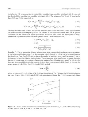
wherewehaveused P = P ∕2 for OOK. Solid and dotted lines in Fig. 7.16 show the BER obtained using
in in
the exact Q-factor (Eqs. (7.131) and (7.132)) and approximate Q-factor (Eq. (7.135)), respectively. Since
10 –5
10 –10 P in = –6 dBm
BER 10 –15

P in = –3 dBm
10 –20

10 –25
50 60 70 80 90 100
No. of amplifiers

Figure 7.16 BER vs. number of amplifiers for direct detection system. Parameters: n = 2, = 0.2 dB/km, amp. spacing
sp
= 80 km, gain G = 16 dB, R = 1000 Ω, T = 200 K, R = 1A/W.
L