Page 340 - Fiber Optic Communications Fund

Transmission System Design 321

the difference between these curves is negligible, the approximation that the variance of receiver noise is
much smaller than that of ASE is good. When spontaneous–spontaneous beat noise is comparable with
signal–spontaneous beat noise, Eq. (7.136) needs to be modified [7–9]. Note that the Gaussian distribu-
tion is an approximation and the amplifier noise after the photodetector is actually chi-square distributed [7]
(see Chapter 8).

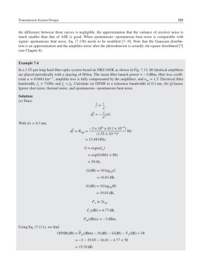
Example 7.4
In a 1.55-μm long-haul fiber-optic system based on NRZ-OOK as shown in Fig. 7.13, 80 identical amplifiers
are placed periodically with a spacing of 80 km. The mean fiber launch power =−3 dBm, fiber loss coeffi-
−1
cient = 0.0461 km , amplifier loss is fully compensated by the amplifiers, and n = 1.5. Electrical filter
sp
bandwidth, f = 7 GHz and f < f . Calculate (a) OSNR in a reference bandwidth of 0.1 nm, (b) Q-factor.
e e 0
Ignore shot noise, thermal noise, and spontaneous–spontaneous beat noise.
Solution:
(a) Since
c
f = ,

c
df =− d.
2
With d = 0.1nm,
8
−9
−3 × 10 ×(0.1 × 10 )
df = B opt = Hz
−6 2
(1.55 × 10 )
= 12.48 GHz,
G = exp(L )
a
= exp(0.0461 × 80)
= 39.96,

G(dB)= 10 log G
10
= 16.01 dB,

N(dB)= 10 log 80
10
= 19.03 dB,

F ≅ 2n ,
n sp
F (dB)= 4.77 dB,
n
P (dBm)=−3dBm.
in
Using Eq. (7.111), we find
OSNR(dB)= P (dBm)− N(dB)− G(dB)− F (dB)+ 58
n
in
=−3 − 19.03 − 16.01 − 4.77 + 58
= 15.19 dB.