Page 450 - Fiber Optic Communications Fund

Nonlinear Effects in Fibers 431

140
40
120
100
30
80
Power (mw) 20 60 δω/2π (GHz)

10 40
20
0 0

–20
–10
–300 –200 –100 0 100 200 300
Time, T (ps)
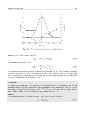
Figure 10.4 Power and instantaneous frequency at the fiber output.

Suppose the input field envelope is given by
√
2
2
q(T, 0)= P exp (−T ∕2T ). (10.94)
0
The instantaneous frequency at L is
( )
2PL T T 2
eff
(T)= exp − . (10.95)
T 2 T 2
0 0
The instantaneous power and frequency at the fiber output are shown in Fig. 10.4. The instantaneous frequency
is negative (or less than the carrier frequency) near the leading edge, whereas it is positive near the trailing
edge. In other words, it is down-shifted in frequency (red shift) near the leading edge and up-shifted (blue
shift) near the trailing edge, as shown in Fig. 10.5.

Example 10.2
In a 1000-km fiber-optic link, it is desired that the peak nonlinear phase shift accumulated over the link
−1
should be less than 0.5 rad. The system has the following parameters: loss coefficient = 0.046 km , ampli-
2
fier spacing = 100 km, Kerr coefficient n = 2.5 × 10 −20 m ∕W, = 1550 nm, and peak power at the fiber
2 0
input = 0 dBm. Find the lower limit on the effective area of the fiber. Ignore .
2
Solution:
The peak nonlinear phase shift accumulated over a single span is given by Eq. (10.91),

= L P , (10.96)
NL eff peak