Page 453 - Fiber Optic Communications Fund

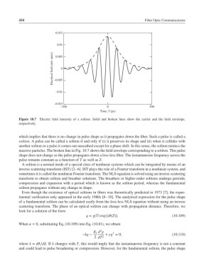
434 Fiber Optic Communications

0.015

0.01

Electrical field (arb. units) –0.005 0
0.005

–0.01

–0.015
–500 0 500
Time, T (ps)

Figure 10.7 Electric field intensity of a soliton. Solid and broken lines show the carrier and the field envelope,
respectively.

which implies that there is no change in pulse shape as it propagates down the fiber. Such a pulse is called a
soliton. A pulse can be called a soliton if and only if (i) it preserves its shape and (ii) when it collides with
another soliton or a pulse it comes out unscathed except for a phase shift. In this sense, the soliton mimics the
massive particles. The broken line in Fig. 10.7 shows the field envelope corresponding to a soliton. This pulse
shape does not change as the pulse propagates down a loss-less fiber. The instantaneous frequency across the
pulse remains constant as a function of T as well as Z.
A soliton is a normal mode of a special class of nonlinear systems which can be integrated by means of an
inverse scattering transform (IST) [2–6]. IST plays the role of a Fourier transform in a nonlinear system, and
sometimes it is called the nonlinear Fourier transform. The NLS equation is solved using an inverse scattering
transform to obtain soliton and breather solutions. The breathers or higher-order solitons undergo periodic
compression and expansion with a period which is known as the soliton period, whereas the fundamental
soliton propagates without any change in shape.
Even though the existence of optical solitons in fibers was theoretically predicted in 1973 [7], the exper-
imental verification only appeared in the early 1980s [8–10]. The analytical expression for the pulse shape
of a fundamental soliton can be calculated easily from the loss-less NLS equation without using an inverse
scattering transform. The phase of an optical soliton can change with propagation distance. Therefore, we
look for a solution of the form
q = g(T) exp [i(Z)]. (10.109)

When = 0, substituting Eq. (10.109) into Eq. (10.81), we obtain
2
d g 3
2
−kg − + g = 0, (10.110)
2 dT 2
where k = d∕dZ.If k changes with T, this would imply that the instantaneous frequency is not a constant
and could lead to pulse broadening or compression. However, for the fundamental soliton, the pulse shape