Page 452 - Fiber Optic Communications Fund

Nonlinear Effects in Fibers 433

From Eq. (10.78), we have
n 0 2n 2 −3 −1 −1
2
= = < 2.32 × 10 W m , (10.106)
cA A
eff 0 eff
2n 2
2
A eff > m , (10.107)
× 2.32 × 10 −3
0
2
A eff > 43.61 μm . (10.108)
2
The effective area should be greater than 43.61 μm to have the peak nonlinear phase shift less than or equal
to 0.5 rad.

10.6 Combined Effect of Dispersion and SPM

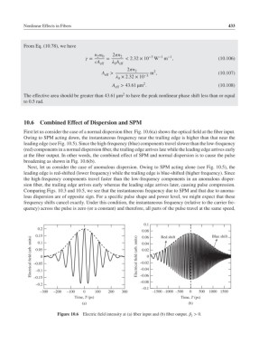
First let us consider the case of a normal dispersion fiber. Fig. 10.6(a) shows the optical field at the fiber input.
Owing to SPM acting down, the instantaneous frequency near the trailing edge is higher than that near the
leading edge (see Fig. 10.5). Since the high-frequency (blue) components travel slower than the low-frequency
(red) components in a normal dispersion fiber, the trailing edge arrives late while the leading edge arrives early
at the fiber output. In other words, the combined effect of SPM and normal dispersion is to cause the pulse
broadening as shown in Fig. 10.6(b).
Next, let us consider the case of anomalous dispersion. Owing to SPM acting alone (see Fig. 10.5), the
leading edge is red-shifted (lower frequency) while the trailing edge is blue-shifted (higher frequency). Since
the high-frequency components travel faster than the low-frequency components in an anomalous disper-
sion fiber, the trailing edge arrives early whereas the leading edge arrives later, causing pulse compression.
Comparing Figs. 10.3 and 10.5, we see that the instantaneous frequency due to SPM and that due to anoma-
lous dispersion are of opposite sign. For a specific pulse shape and power level, we might expect that these
frequency shifts cancel exactly. Under this condition, the instantaneous frequency (relative to the carrier fre-
quency) across the pulse is zero (or a constant) and therefore, all parts of the pulse travel at the same speed,

0.1
0.2
0.08
0.15 0.06 Red shift Blue shift
Electrical field (arb. units) –0.05 0 Electrical field (arb. units) –0.02 0
0.1
0.04
0.05
0.02

–0.04
–0.1
–0.06
–0.15
–0.08
–0.2
–0.1
–300 –200 –100 0 100 200 300 –1500 –1000 –500 0 500 1000 1500
Time, T (ps) Time, T (ps)
(a) (b)
Figure 10.6 Electric field intensity at (a) fiber input and (b) fiber output. > 0.
2