Page 456 - Fiber Optic Communications Fund

Nonlinear Effects in Fibers 437

10.7 Interchannel Nonlinear Effects
So far we have considered the modulation of a single optical carrier. In a wavelength-division multiplexing
system (see Chapter 9), multiple carriers are modulated by electrical data and, in this case, the nonlinear
Schrödinger equation is valid if the total spectral width is much smaller than the reference carrier frequency.
Typically, the spectral width of a WDM signal is about 3 to 4 THz, which is much smaller than the carrier
frequency of 194 THz corresponding to the center of the erbium window. The total optical field may be
written as
N∕2−1
∑ −i( n t− n z)
Ψ= q (t, z)e , (10.128)
n
n=−N∕2
where and q (t, z) are the carrier frequency and the slowly varying envelope of the nth channel, respectively,
n n
and N is the number of channels. Eq. (10.128) may be rewritten as
Ψ= qe −i( 0 t− 0 z) , (10.129)

where
N∕2−1
∑ −i(Ω n t− n z)
q = q (t, z)e (10.130)
n
n=−N∕2
and Ω ≡ − is the relative center frequency of channel n with respect to a reference frequency ,
n n 0 0
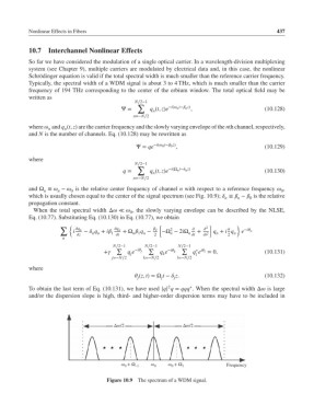
which is usually chosen equal to the center of the signal spectrum (see Fig. 10.9); ≡ − is the relative
n n 0
propagation constant.
When the total spectral width Δ≪ , the slowly varying envelope can be described by the NLSE,
0
Eq. (10.77). Substituting Eq. (10.130) in Eq. (10.77), we obtain
∑ { [ 2 ] }
2
i q n − q + i q n +Ω q − 2 −Ω − 2iΩ + q + i q e −i n
z n n 1 t n 1 n 2 n n t t 2 n 2 n
n
N∕2−1 N∕2−1 N∕2−1
∑ ∑ ∑ ∗ i
+ q e −i j q e −i k q e l = 0, (10.131)
k
j
l
j=−N∕2 k=−N∕2 l=−N∕2
where
(z, t)=Ω t − z. (10.132)
j
j
j
∗
2
To obtain the last term of Eq. (10.131), we have used |q| q = qqq . When the spectral width Δ is large
and/or the dispersion slope is high, third- and higher-order dispersion terms may have to be included in
Δω/2 Δω/2

ω 0 + Ω –1 ω 0 ω 0 + Ω 1 Frequency

Figure 10.9 The spectrum of a WDM signal.