Page 485 - Fiber Optic Communications Fund

466 Fiber Optic Communications

∞
√ ∑
I lin ≈ 2 P 0 b u lin,n , (10.308)
n
n=−∞,n≠0
√ ∑
I ≈ 2 P b b b Re(u ). (10.309)
nl 0 l m n lmn
l+m−n=0
The variance is calculated as (see Example 10.14)
2 2 2
=< I > − < I> (10.310)
OOK
2
= 2 + , (10.311)
lin nl
where
∞ ( 2 2 )
∑ −m T s
2
= P 0 exp , (10.312)
lin 2
m=−∞ T 0
( )
∑ ∑ 1 1
2
2
= 4 P − Re(u )Re(u ′ m ′ n ′). (10.313)
nl 0 x(l,m,n,l ′ ,m ′ ,n ′ ) r(l,m,n)−r(l ′ ,m ′ ,n ′ ) lmn l
l+m−n=0 l ′ +m ′ −n ′ =0 2 2
′
′
′
r(l, m, n) is the number of non-degenerate indices in the set {l, m, n} and x(l, m, n, l , m , n ) is the number of
′
′
′
non-degenerate indices in the set {l, m, n, l , m , n }.
10.9.2 Numerical Simulations
To test the accuracy of the semi-analytical expressions for the variance, numerical simulation of the NLSE
is carried out using the symmetric split-step Fourier scheme (see Chapter 11). The fiber-optic link is shown
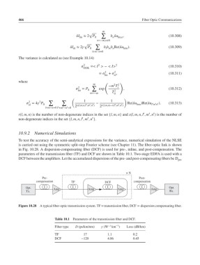
in Fig. 10.28. A dispersion-compensating fiber (DCF) is used for pre-, inline, and post-compensation. The
parameters of the transmission fiber (TF) and DCF are shown in Table 10.1. Two-stage EDFA is used with a
DCF between the amplifiers. Let the accumulated dispersions of the pre- and post-compensating fibers be  pre
× N
Pre- Post-
compensation TF DCF compensation
Opt. Amp Amp Amp Amp Opt.
Tx. Rx.

Figure 10.28 A typical fiber-optic transmission system. TF = transmission fiber, DCF = dispersion compensating fiber.

Table 10.1 Parameters of the transmission fiber and DCF.
−1
Fiber type D (ps/km/nm) (W −1 km ) Loss (dB/km)
TF 17 1.1 0.2
DCF −120 4.86 0.45