Page 68 - Fiber Optic Communications Fund

Optical Fiber Transmission 49

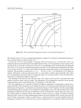
Figure 2.16 Plot of normalized propagation constant b versus normalized frequency V.

The solutions of Eq. (2.57) for a normalized propagation constant b as a function of normalized frequency V
give us universal curves as shown in Fig. 2.16.
To solve Eq. (2.57), we first calculate V using Eq. (2.59). Let us first set m = 0. Since Eq. (2.57) is an
implicit function of b, the left-hand side and right-hand side of Eq. (2.57) are plotted for various values of b in
the interval [0, 1]. The point of intersection of the curves corresponding to the left-hand side and right-hand
side of Eq. (2.57) gives the normalized propagation constant b of the guided mode supported by the fiber.
As can be seen from Fig. 2.17, there can be many intersections which means there are several guided-mode
solutions. This procedure is repeated for m = 1, 2, … , M.For m = M + 1, we find that Eq. (2.57) admits no
solution. When there is only one intersection (M = 1), such a fiber is called a single-mode fiber. The values
of b corresponding to the intersections for a particular value of V are shown in Fig. 2.16 by the broken lines.
This process is repeated for different values of V.
The advantage of the universal curve shown in Fig. 2.16 is that it can be used for a step-index fiber with
arbitrary refractive indices and core radius. The dependence of the propagation constant on the specific
design parameter can be extracted from Fig. 2.16 using Eqs. (2.58) and (2.59).
For many applications, it is required to obtain the frequency dependence of propagation constant in a
single-mode fiber. This information can be obtained from Fig. 2.16. For the given fiber parameters and for the
desired range of frequencies, V-parameters are calculated using Eq. (2.59). Using Fig. 2.16, the corresponding
normalized propagation constants, b are calculated (corresponding to LP ) and with the help of Eq. (2.58),
01
propagation constants for this range of frequencies can be calculated. For a specific value of m, Eq. (2.57)
has a finite number of solutions and the nth solution is known as the LP mn mode. LP stands for linearly
polarized mode. Under the weakly guiding approximation, the electromagnetic field is nearly transverse and
each LP mode corresponds to either an x-polarized or a y-polarized mode. For an ideal cylindrical fiber, the
propagation constants of the x-polarized LP mn and the y-polarized LP mn are identical. When the refractive