Page 70 - Fiber Optic Communications Fund

Optical Fiber Transmission 51

where and are the characteristic impedances of core and cladding, respectively. F mn can be determined
1
2
after performing the integrations in Eq. (2.64) numerically. Eq. (2.61) can be normalized so that the power
carried by this mode is unity,
1
P tot = 1 or C = √ (2.65)
1
F
mn
and
= R (r)e −i(t− mn z−im) , (2.66)
mn
where
{ ( ) √
J m r ∕ F mn for r ≤ a
1
R (r)= √ . (2.67)
mn
[J ( a)∕K ( a)]K ( r)∕ F for r > a
m 1 m 2 m 2 mn
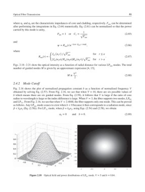
Figs. 2.18–2.21 show the optical intensity as a function of radial distance for various LP mn modes. The total
number of guided modes M is given by an approximate expression [4, 13],
V 2
M ≅ . (2.68)
2
2.4.2 Mode Cutoff

Fig. 2.16 shows the plot of normalized propagation constant b as a function of normalized frequency V
obtained by solving Eq. (2.57). From Fig. 2.16, we see that when V = 10, there are six possible values of
b which means there are six guided modes. From Eq. (2.59), it follows that V is large if the ratio of core
radius to wavelength is large or the index difference is large. When V = 3, the fiber supports two modes, LP
01
and LP . From Fig. 2.16, we see that when V < 2.4048, the fiber supports only one mode. This can be proved
11
as follows. Any LP mode ceases to exist when b < 0 because it then corresponds to a radiation mode, since
mn
< k n (Eq. (2.58)). For LP mode, when = k n , using Eqs. (2.54) and (2.58), we obtain
0 2 11 0 2
= 0 and b = 0. (2.69)
2

1
0.8
0.6
0.4
0.2
0
–0.2
–0.4
–0.6
–0.8
–1
–1 –0.5 0 0.5 1

Figure 2.18 Optical field and power distributions of LP mode. V = 5and b = 0.84.
01