Page 380 - Six Sigma Advanced Tools for Black Belts and Master Black Belts

OTE/SPH
OTE/SPH
Char Count= 0
3:8
August 31, 2006
JWBK119-23
Proposed Monitoring Procedure 365
Observations (yt) Residuals
10
A 4 B UCL = +3
5
2
0 0
−2
−5
UCL = −3
−4
−10
0 25 50 75 100 125 150 175 200 225 200 205 210 215 220 225 230
TIME TIME
CUSUM on Residuals Maximum Lambda
30 5.5
C D
25 5
20 h = 17.75, k = 0.05 4.5
15 4
10 3.5 UCL = 3.43
5 3
0 2.5
200 205 210 215 220 225 230 200 205 210 215 220 225 230
TIME TIME
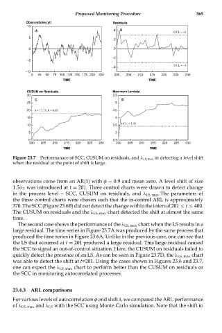
Figure 23.7 Performanace of SCC, CUSUM on residuals, and λ LS,max in detecting a level shift
when the residual at the point of shift is large.

observations come from an AR(1) with φ = 0.9 and mean zero. A level shift of size
1.5σ Z was introduced at t = 201. Three control charts were drawn to detect change
in the process level -- SCC, CUSUM on residuals, and λ LS, max .The parameters of
the three control charts were chosen such that the in-control ARL is approximately
370.TheSCC(Figure23.6B)didnotdetectthechangewithintheinterval201 ≤ t ≤ 400.
The CUSUM on residuals and the λ LS, max chart detected the shift at almost the same
time.
The second case shows the performance of the λ LS, max chart when the LS results in a
large residual. The time series in Figure 23.7A was produced by the same process that
produced the time series in Figure 23.6A. Unlike in the previous case, one can see that
the LS that occurred at t = 201 produced a large residual. This large residual caused
the SCC to signal an out-of-control situation. Here, the CUSUM on residuals failed to
quickly detect the presence of an LS. As can be seen in Figure 23.7D, the λ LS, max chart
was able to detect the shift at t=201. Using the cases shown in Figures 23.6 and 23.7,
one can expect the λ LS, max chart to perform better than the CUSUM on residuals or
the SCC in monitoring autocorrelated processes.

23.4.3 ARL comparisons
For various levels of autocorrelation φ and shift δ, we compared the ARL performance
of λ LS, max and ¯ λ LS with the SCC using Monte Carlo simulation. Note that the shift in