Page 377 - Six Sigma Advanced Tools for Black Belts and Master Black Belts

OTE/SPH
OTE/SPH
3:8
August 31, 2006
Char Count= 0
JWBK119-23
362 Statistical Process Control for Autocorrelated Processes
Lambda (LS, t)
3
2
1

0
−1
−2
−3
0 10 20 30 40 50 60 70 80 90 100
TIME (t)
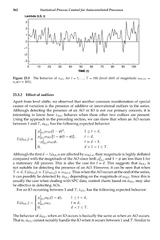
Figure 23.5 The behavior of λ LS,t for t = 1,..., T = 100 (level shift of magnitude ω LS,101 =
σ z at t = 101).

23.3.2 Effect of outliers
Apart from level shifts, we observed that another common manifestation of special
causes of variation is the presence of additive or innovational outliers in the series.
Although detecting the presence of an AO or IO is not our primary concern, it is
interesting to know how λ LS,t behaves when these other two outliers are present.
Using the approach in the preceding section, we can show that when an AO occurs
between 1 and T,ˆω LS,t has the following expected behavior:

⎧ 2 2
⎪ ρ ω AO (1 − φ) , 1 ≤ t < d,
⎪ LS,t
⎪ 2
ρ LS,t ω AO [1 − φ(1 − φ)] , t = d,
⎨
E(ˆω LS,t ) = 2
⎪ −ρ LS,t ω AO φ, t = d + 1,
⎪
⎪
0, d + 1 < t ≤ T.
⎩
Although the first d − 1ˆω LS,t s are affected by ω AO,d , their magnitude is highly deflated
2
compared with the magnitude of the AO since both ρ LS,t and 1 − φ are less than 1 for
a stationary AR process. This is also the case for t = d. This suggests that ˆω LS,t is
not suitable for detecting the presence of an AO. However, it can be seen that when
T = d, E(ˆω LS,d ) = E(ˆω AO,d ) = ω AO,d . Thus when the AO occurs at the end of the series,
it can possibly be detected by ˆω LS,t depending on the magnitude of ω AO . Since this is
usually the case when dealing with SPC data, control charts based on ˆω LS,t may also
be effective in detecting AOs.
For an IO occurring between 1 and T, λ LS,t has the following expected behavior:
⎧ 2
⎪ ρ ω IO (1 − φ), 1 ≤ t < d,
⎨ LS,t
2
E(ˆω LS,t ) = ρ LS,t ω IO , t = d,
⎪
⎩ 0, d < t ≤ T.
The behavior of ˆω LS,t when an IO occurs is basically the same as when an AO occurs.
That is, ˆω LS,t cannot suitably handle the IO when it occurs between 1 and T. Similar to