Page 372 - Six Sigma Advanced Tools for Black Belts and Master Black Belts

OTE/SPH
OTE/SPH
Char Count= 0
August 31, 2006
3:8
JWBK119-23
Detecting Outliers and Level Shifts 357
(d)
If we let y t = [φ(B)/θ(B)]Y t and x t = [φ(B)ω(B)/θ(B)δ(B)]ξ t , we have
y t = ω 0 x t + ε t ,
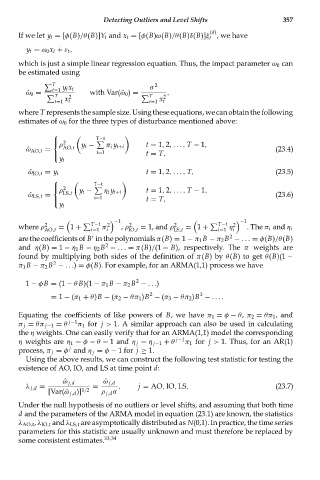
which is just a simple linear regression equation. Thus, the impact parameter ω 0 can
be estimated using
T 2
t=1 y t x t σ ,
T 2 with Var( ˆω 0 ) = T 2
ˆ ω 0 =
t=1 x t t=1 x t
where T representsthesamplesize.Usingtheseequations,wecanobtainthefollowing
estimates of ω 0 for the three types of disturbance mentioned above:

T−t
⎧

⎨ 2
ρ y t − π i y t+i t = 1, 2,..., T − 1,
ˆ ω AO,t = AO,t (23.4)
i=1 t = T,
⎩
y t
ˆ ω IO,t = y t t = 1, 2,..., T, (23.5)
⎧
T−t

⎨ 2
ρ y t − η i y t+i t = 1, 2,..., T − 1,
ˆ ω LS,t = LS,t (23.6)
i=1
⎩ t = T,
y t
−1 −1
where ρ 2 = 1 + T−t π 2 , ρ 2 = 1, and ρ 2 = 1 + T−t η 2
AO,t i=1 i IO,t LS,t i=1 i . The π i and η i
2
i
are the coefficients of B in the polynomials π(B) = 1 − π 1 B − π 2 B − ... = φ(B)/θ(B)
2
and η(B) = 1 − η 1 B − η 2 B − ... = π(B)/(1 − B), respectively. The π weights are
found by multiplying both sides of the definition of π(B)by θ(B)toget θ(B)(1 −
2
π 1 B − π 2 B − ...) = φ(B). For example, for an ARMA(1,1) process we have
2
1 − φB = (1 − θ B)(1 − π 1 B − π 2 B − ...)
2
3
= 1 − (π 1 + θ)B − (π 2 − θπ 1 )B − (π 3 − θπ 2 )B − ....
Equating the coefficients of like powers of B, we have π 1 = φ − θ, π 2 = θπ 1 , and
π j = θπ j−1 = θ j−1 π 1 for j > 1. A similar approach can also be used in calculating
the η weights. One can easily verify that for an ARMA(1,1) model the corresponding
η weights are η 1 = φ − θ − 1 and η j = η j−1 + θ j−1 π 1 for j > 1. Thus, for an AR(1)
j
process, π j = φ and η j = φ − 1 for j ≥ 1.
Using the above results, we can construct the following test statistic for testing the
existence of AO, IO, and LS at time point d:
ˆ ω j,d ˆ ω j,d
λ j,d = = , j = AO, IO, LS. (23.7)
[Var( ˆω j,d )] 1/2 ρ j,d σ
Under the null hypothesis of no outliers or level shifts, and assuming that both time
d and the parameters of the ARMA model in equation (23.1) are known, the statistics
λ AO,t , λ IO,t and λ LS,t are asymptotically distributed as N(0,1). In practice, the time series
parameters for this statistic are usually unknown and must therefore be replaced by
some consistent estimates. 33,34