Page 371 - Six Sigma Advanced Tools for Black Belts and Master Black Belts

OTE/SPH
OTE/SPH
3:8
August 31, 2006
Char Count= 0
JWBK119-23
356 Statistical Process Control for Autocorrelated Processes
Zt Yt
6 6
A B
4 4
2 2
0 0
−2 −2
−4 −4
0 20 40 60 80 100 0 20 40 60 80 100
TIME (t) TIME (t)

Yt Yt
6 6
C D
4 4
2 2
0 0
−2 −2
−4 −4
0 20 40 60 80 100 0 20 40 60 80 100
TIME (t) TIME (t)

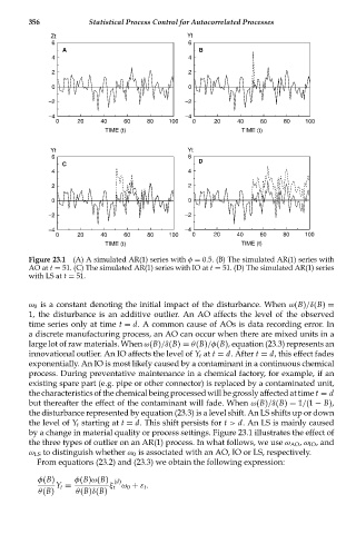
Figure 23.1 (A) A simulated AR(1) series with φ = 0.5. (B) The simulated AR(1) series with
AO at t = 51. (C) The simulated AR(1) series with IO at t = 51. (D) The simulated AR(1) series
with LS at t = 51.

ω 0 is a constant denoting the initial impact of the disturbance. When ω(B)/δ(B) =
1, the disturbance is an additive outlier. An AO affects the level of the observed
time series only at time t = d. A common cause of AOs is data recording error. In
a discrete manufacturing process, an AO can occur when there are mixed units in a
large lot of raw materials. When ω(B)/δ(B) = θ(B)/φ(B), equation (23.3) represents an
innovational outlier. An IO affects the level of Y t at t = d. After t = d, this effect fades
exponentially. An IO is most likely caused by a contaminant in a continuous chemical
process. During preventative maintenance in a chemical factory, for example, if an
existing spare part (e.g. pipe or other connector) is replaced by a contaminated unit,
the characteristics of the chemical being processed will be grossly affected at time t = d
but thereafter the effect of the contaminant will fade. When ω(B)/δ(B) = 1/(1 − B),
the disturbance represented by equation (23.3) is a level shift. An LS shifts up or down
the level of Y t starting at t = d. This shift persists for t > d. An LS is mainly caused
by a change in material quality or process settings. Figure 23.1 illustrates the effect of
the three types of outlier on an AR(1) process. In what follows, we use ω AO , ω IO , and
ω LS to distinguish whether ω 0 is associated with an AO, IO or LS, respectively.
From equations (23.2) and (23.3) we obtain the following expression:
φ(B) φ(B)ω(B) (d)
Y t = ξ t ω 0 + ε t .
θ(B) θ(B)δ(B)