Page 366 - Six Sigma Advanced Tools for Black Belts and Master Black Belts

OTE/SPH
OTE/SPH
Char Count= 0
August 31, 2006
3:7
JWBK119-22
Conclusion 351
MH-statistic
25
20
UCL=16.32
15

10
5

0
0 100 200 300 400 500
Time (t)
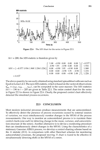
Figure 22.6 The MH chart for the series in Figure 22.5.

At t = 200, the MH-statistic is therefore given by

1.00 −0.90 0.00 0.00 0.00 −0.577
⎡ ⎤ ⎡ ⎤
⎢ −0.90 1.81 −0.90 0.00 0.00 ⎥ ⎢ 1.934 ⎥
⎢ ⎥ ⎢ ⎥
MH = [ −0.577 1.934 1.968 1.234 1.224 ] ⎢ 0.00 −0.90 1.81 −0.90 0.00 ⎥ ⎢ 1.968 ⎥
0.00 0.00 −0.90 1.81 −0.90 1.234
⎣ ⎦ ⎣ ⎦
0.00 0.00 0.00 −0.90 1.00 1.224
= 6.437
Theabovequantitybecaneasilyobtainedusingstandardspreadsheetsoftwaresuchas
Excel or Lotus1-2-3. The next MH-statistic, which is based on the vector of observations

x * 201 = (x 197 , x 198 ,..., x 201 ) , can be computed in the same manner. The MH statistics
for t = 196 to t = 205 are given in Table 22.1. The entire control chart for the series
in Figure 22.5 is shown in Figure 22.6. Clearly, the proposed control chart effectively
detected the simulated process excursions.

22.5 CONCLUSION

Most modern industrial processes produce measurements that are autocorrelated.
To effectively detect the presence of process excursions caused by external sources
of variation, we must simultaneously monitor changes in the MVAS of the process
measurements. One way to monitor an autocorrelated process is to maintain three
control charts (one each for detecting change in the mean, variance, and autocorrela-
tion structure of the series). Another alternative is to devise a monitoring procedure
that can simultaneously detect changes in the MVAS. Using the characteristics of a
stationary Gaussian ARMA process, we develop a control-charting scheme based on
the H statistic (22.1). In comparison with other Shewhart schemes for monitoring
autocorrelated processes, the proposed moving H chart is found to be effective in
simultaneously detecting shifts in the MVAS of a series.