Page 364 - Six Sigma Advanced Tools for Black Belts and Master Black Belts

OTE/SPH
OTE/SPH
3:7
August 31, 2006
JWBK119-22
Char Count= 0
Numerical Example 349
500 500
AR1 = 0.0 AR1 = 0.9
200 SACC 200
100 100
50 50
ARL ARL
20 20
SCC
10 10
MH (5)
5 5
2 2
1 1.5 2 2.5 3 1 1.5 2 2.5 3
Change in Variance Change in Variance
Figure 22.3 Sensitivity of the SCC, SACC and MH chart in delecting shifts in the variance.

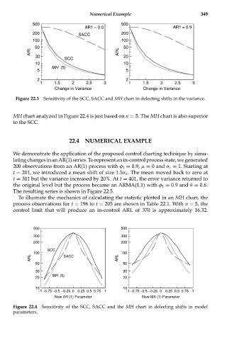
MH chart analyzed in Figure 22.4 is just based on n = 5. The MH chart is also superior
to the SCC.

22.4 NUMERICAL EXAMPLE

We demonstrate the application of the proposed control charting technique by simu-
latingchangesinanAR(1)series.Torepresentanin-controlprocessstate,wegenerated
200 observations from an AR(1) process with φ 1 = 0.9, μ = 0 and σ ε = 1. Starting at
t = 201, we introduced a mean shift of size 1.5σ x . The mean moved back to zero at
t = 301 but the variance increased by 20%. At t = 401, the error variance returned to
the original level but the process became an ARMA(1,1) with φ 1 = 0.9 and θ = 0.6.
The resulting series is shown in Figure 22.5.
To illustrate the mechanics of calculating the statistic plotted in an MH chart, the
process observations for t = 196 to t = 205 are shown in Table 22.1. With n = 5, the
control limit that will produce an in-control ARL of 370 is approximately 16.32.

500 500
300 300
200 200
SCC
100 100
ARL SACC ARL
50 50
30 30
MH (5)
20 20
10 10
−1 −0.75 −0.5 −0.25 0 0.25 0.5 0.75 1 −1 −0.75 −0.5 −0.25 0 0.25 0.5 0.75 1
New AR (1) Parameter New MA (1) Parameter

Figure 22.4 Sensitivity of the SCC, SACC and the MH chart in delecting shifts in model
parameters.