Page 360 - Six Sigma Advanced Tools for Black Belts and Master Black Belts

OTE/SPH
OTE/SPH
JWBK119-22
August 31, 2006
Char Count= 0
3:7
The Proposed Approach 345
characteristics of a stationary Gaussian process, is much simpler to implement and is
sensitive to shifts in the MVAS of a series. Although the proposed procedure can be
implemented for the general ARMA case, we will focus our analysis on the important
case of AR(1) process. The importance of the AR(1) process in process control has been
emphasized in the literature. 2,10−12

22.2 THE PROPOSED APPROACH

We follow the usual assumption that when the process is stable, the sequence of
process measurements {x t } can be modeled as a stationary Gaussian ARMA(p, q)
process

φ p (B)x t = φ 0 + θ q (B)ε t ,
where {x t } is a stationary time series representing the process measurements,
2
φ p (B) = 1 − φ 1 B − φ 2 B − ··· − φ p B p
is an autoregressive polynomial of order p,
2
θ q (B) = 1 − θ 1 B − θ 2 B − ··· − θ q B q
is a moving average polynomial of order q, B is the backshift operator, and {ε t } is a
sequence of normally and independently distributed random errors with mean zero
2
and constant variance σ . Without loss of generality, we assume that the level φ 0 of
ε
the in-control process measurements is zero.
By definition, if {x t , t = 1, 2, 3,...} is a stationary Gaussian process then {x t } is
strictly stationary, since for all n ∈{1, 2,...} and for all h, t 1 , t 2 ,... ∈ Z, the random
) and (x t 1 +h ,..., x t n +h ) have the same mean and covariance matrix,

vectors (x t t ,..., x t n
13
and hence the same distribution (see p. 13 of Brockwell and Davis ). Let {x t } be a sta-
) is multivariate normal with

tionary Gaussian ARMA process. Then x = (x t 1 ,..., x t n
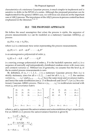
mean μ 0 and covariance matrix
⎡ ⎤ ⎡ ⎤
... 1 ...
γ 0 γ 1 γ 2 γ n−1 ρ 1 ρ 2 ρ n−1
... 1 ...
γ 1 γ 0 γ 1 γ n−2 ρ 1 ρ 1 ρ n−2
⎢ ⎥ ⎢ ⎥
⎢ ⎥ ⎢ ⎥
⎢ γ 2 γ 1 γ 0 ... γ n−3 ⎥ ⎢ ρ 2 ρ 1 1 ... ρ n−3 ⎥
⎢ ⎥ ⎢ ⎥
0 = ⎢ . . . . . ⎥ = σ 2 ⎢ . . . . ⎥ ,
⎢ ⎥ x ⎢ ⎥
. . . . . . . . . . . . . .
⎢ ⎥ ⎢ ⎥
⎢ ⎥ ⎢ ⎥
⎣ . . . . ⎦ ⎣ . . . . ⎦
γ n−1 γ n−2 γ n−3 ... γ 0 ρ n−1 ρ n−2 ρ n−3 ... 1
where γ k and ρ k represent the autocovariance and autocorrelation at lag k, respectively.
For an ARMA (1,1) process the autocovariance function is given by
2
1 + θ − 2φ 1 θ 1 2
1
γ 0 = 2 σ ,
ε
1 − φ
1
(1 − φ 1 θ 1 )(φ 1 − θ 1 ) 2
γ 1 = 2 σ ,
ε
1 − φ 1
γ k = φ 1 γ k−1 , k ≥ 2,