Page 375 - Six Sigma Advanced Tools for Black Belts and Master Black Belts

OTE/SPH
OTE/SPH
August 31, 2006
3:8
JWBK119-23
Char Count= 0
360 Statistical Process Control for Autocorrelated Processes
Observations (Yt)
8
6
4
2
0
−2
−4
−6
−8
0 25 50 75 100 125 150 175 200 225 250 275 300
TIME (t)

2
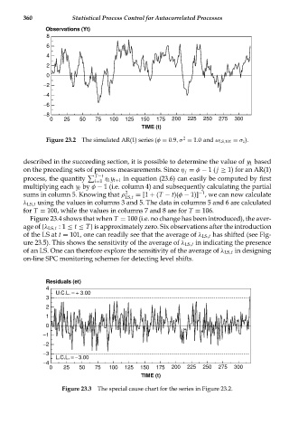
Figure 23.2 The simulated AR(1) series (φ = 0.9,σ = 1.0 and ω LS,101 = σ z ).

described in the succeeding section, it is possible to determine the value of y 1 based
on the preceding sets of process measurements. Since η j = φ − 1( j ≥ 1) for an AR(1)
T−t
process, the quantity i=1 η i y t+i in equation (23.6) can easily be computed by first
multiplying each y t by φ − 1 (i.e. column 4) and subsequently calculating the partial
−1
sums in column 5. Knowing that ρ 2 = [1 + (T − t)(φ − 1)] , we can now calculate
LS,t
λ LS,t using the values in columns 3 and 5. The data in columns 5 and 6 are calculated
for T = 100, while the values in columns 7 and 8 are for T = 106.
Figure 23.4 shows that when T = 100 (i.e. no change has been introduced), the aver-
age of {λ LS,t :1 ≤ t ≤ T} is approximately zero. Six observations after the introduction
of the LS at t = 101, one can readily see that the average of λ LS,t has shifted (see Fig-
ure 23.5). This shows the sensitivity of the average of λ LS,t in indicating the presence
of an LS. One can therefore explore the sensitivity of the average of λ LS,t in designing
on-line SPC monitoring schemes for detecting level shifts.

Residuals (et)
4
U.C.L. = + 3.00
3
2
1
0
−1
−2
−3
L.C.L. = − 3.00
−4
0 25 50 75 100 125 150 175 200 225 250 275 300
TIME (t)
Figure 23.3 The special cause chart for the series in Figure 23.2.