Page 374 - Six Sigma Advanced Tools for Black Belts and Master Black Belts

OTE/SPH
OTE/SPH
Char Count= 0
3:8
August 31, 2006
JWBK119-23
359
Behavior of λ LS,t
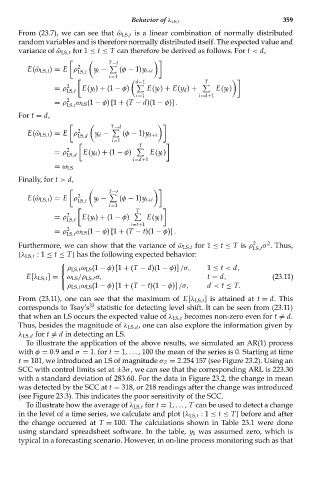
From (23.7), we can see that ˆω LS,t is a linear combination of normally distributed
random variables and is therefore normally distributed itself. The expected value and
variance of ˆω LS,t for 1 ≤ t ≤ T can therefore be derived as follows. For t < d,

T−t
E(ˆω LS,t ) = E ρ 2 y t −
LS,t (φ − 1)y t+i
i=1
d−1 T

= ρ 2 E(y t ) + (1 − φ) E(y i ) + E(y d ) + E(y i )
LS,t
i=1 i=d+1
= ρ 2 ω LS (1 − φ) [1 + (T − d)(1 − φ)] .
LS,t
For t = d,
T−d

E(ˆω LS,t ) = E ρ 2 y d − (φ − 1)y d+i
LS,d
i=1
T

= ρ 2 E(y d ) + (1 − φ) E(y i )
LS,d
i=d+1
= ω LS
Finally, for t > d,
T−t

E(ˆω LS,t ) = E ρ 2 y t −
LS,t (φ − 1)y t+i
i=1
T

= ρ 2 E(y t ) + (1 − φ) E(y i )
LS,t
i=t+1
= ρ 2 ω LS (1 − φ) [1 + (T − t)(1 − φ)] .
LS,t
2
2
Furthermore, we can show that the variance of ˆω LS,t for 1 ≤ t ≤ T is ρ LS,t σ . Thus,
{λ LS,t :1 ≤ t ≤ T} has the following expected behavior:
⎧
⎨ ρ LS,t ω LS (1 − φ) [1 + (T − d)(1 − φ)] /σ, 1 ≤ t < d,
E[λ LS,t ] = ω LS /ρ LS,t σ, t = d, (23.11)
ρ LS,t ω LS (1 − φ) [1 + (T − t)(1 − φ)] /σ, d < t ≤ T.
⎩
From (23.11), one can see that the maximum of E[λ LS,t ] is attained at t = d. This
corresponds to Tsay’s 33 statistic for detecting level shift. It can be seen from (23.11)
that when an LS occurs the expected value of λ LS,t becomes non-zero even for t = d.
Thus, besides the magnitude of λ LS,d , one can also explore the information given by
λ LS,d for t = d in detecting an LS.
To illustrate the application of the above results, we simulated an AR(1) process
with φ = 0.9 and σ = 1. for t = 1, . . . , 100 the mean of the series is 0. Starting at time
t = 101, we introduced an LS of magnitude σ Z = 2.254 157 (see Figure 23.2). Using an
SCC with control limits set at ±3σ, we can see that the corresponding ARL is 223.30
with a standard deviation of 283.60. For the data in Figure 23.2, the change in mean
was detected by the SCC at t = 318, or 218 readings after the change was introduced
(see Figure 23.3). This indicates the poor sensitivity of the SCC.
To illustrate how the average of λ LS,t for t = 1, ..., T can be used to detect a change
in the level of a time series, we calculate and plot {λ LS,t :1 ≤ t ≤ T} before and after
the change occurred at T = 100. The calculations shown in Table 23.1 were done
using standard spreadsheet software. In the table, y 1 was assumed zero, which is
typical in a forecasting scenario. However, in on-line process monitoring such as that