Page 379 - Six Sigma Advanced Tools for Black Belts and Master Black Belts

OTE/SPH
OTE/SPH
August 31, 2006
3:8
JWBK119-23
Char Count= 0
364 Statistical Process Control for Autocorrelated Processes
appropriate control limits. This can be done by first specifying a standard or accept-
able in-control ARL. A simulation program is then used to determine what control
limits can be used to achieve this in-control ARL value. For the control chart based on
λ LS,max , the results of Chen and Liu 35 can be used as starting points for simulation.
23.4.2 Control chart performance

For an AR(1) process with φ> 0, when a level shift of magnitude ω LS occurrs at t = d,
the expected value of the residual at that point in time is ω LS . For t > d, the expected
value of the residuals becomes (1 − φ)ω LS . Thus, an SCC has a high chance of detecting
the shift right after it occurs. After this point, the probability of an SCC detecting this
shift becomes small, especially when φ → 1. An SCC is, therefore, expected to give
better performance than a CUSUM chart on residuals when the change in level at time
t = d produces a large residual (e.g. greater than 3 in absolute value). However, given
non-detection of the change in level by the SCC at t = d, use of the CUSUM would be
recommended. Thus, both charts have advantages and disadvantages in monitoring
autocorrelated processes.
The proposed control chart based on λ LS,t combines the desirable properties of
the SCC and the CUSUM. It detects both abrupt and small shifts in process level.
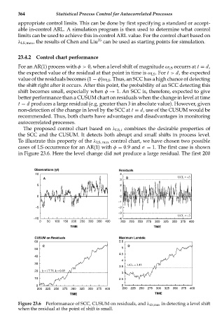
To illustrate this property of the λ LS, max control chart, we have chosen two possible
cases of LS occurrence for an AR(1) with φ = 0.9 and σ = 1. The first case is shown
in Figure 23.6. Here the level change did not produce a large residual. The first 200

Observations (yt) Residuals
10 4
A 3 B UCL = +3
5 2
1
0 0
−1
−5 −2
−3
UCL = −3
−10 −4
0 50 100 150 200 250 300 350 400 200 225 250 275 300 325 350 375 400
TIME TIME
CUSUM on Residuals Maximum Lambda
60 5.5
C D
50 5
4.5
40
4
30
3.5 UCL = 3.43
20 h = 17.75, k = 0.05
3
10 2.5
0 2
200 225 250 275 300 325 350 375 400 200 225 250 275 300 325 350 375 400
TIME TIME
Figure 23.6 Performanace of SCC, CUSUM on residuals, and λ LS,max in detecting a level shift
when the residual at the point of shift is small.