Page 387 - Six Sigma Advanced Tools for Black Belts and Master Black Belts

OTE/SPH
OTE/SPH
3:8
August 31, 2006
JWBK119-24
Char Count= 0
372 Cumulative Sum Charts with Fast Initial Response
Tabular CUSUM Chart
8
6 4
Cumulative Sum 2 0

−2
−4
−6
0 2 4 6 8 10 12 14 16
Sample

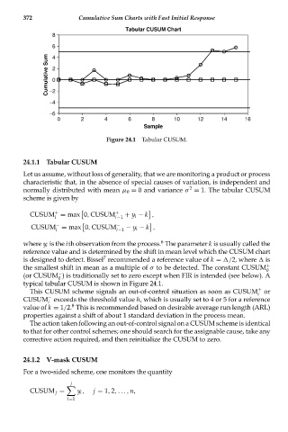
Figure 24.1 Tabular CUSUM.

24.1.1 Tabular CUSUM
Let us assume, without loss of generality, that we are monitoring a product or process
characteristic that, in the absence of special causes of variation, is independent and
2
normally distributed with mean μ 0 = 0 and variance σ = 1. The tabular CUSUM
scheme is given by

+
CUSUM = max 0, CUSUM + + y i − k ,
i i−1

CUSUM = max 0, CUSUM − − y i − k ,
−
i i−1
6
where y i is the ith observation from the process. The parameter k is usually called the
reference value and is determined by the shift in mean level which the CUSUM chart
7
is designed to detect. Bissel recommended a reference value of k = /2, where is
the smallest shift in mean as a multiple of σ to be detected. The constant CUSUM +
0
−
(or CUSUM ) is traditionally set to zero except when FIR is intended (see below). A
0
typical tabular CUSUM is shown in Figure 24.1.
+
This CUSUM scheme signals an out-of-control situation as soon as CUSUM or
i
−
CUSUM exceeds the threshold value h, which is usually set to 4 or 5 for a reference
i
8
value of k = 1/2. This is recommended based on desirable average run length (ARL)
properties against a shift of about 1 standard deviation in the process mean.
The action taken following an out-of-control signal on a CUSUM scheme is identical
to that for other control schemes; one should search for the assignable cause, take any
corrective action required, and then reinitialize the CUSUM to zero.
24.1.2 V-mask CUSUM
For a two-sided scheme, one monitors the quantity
j

CUSUM j = y i , j = 1, 2,..., n,
i=1