Page 399 - Maxwell House

DISCONTINUITY IN FEED LINES 379

analysis with normalized or denormalized - and -matrix since their elements have a tendency
to take an infinite values around the unknown in advance circuit resonances. We hope that the
reader will share our opinion that S-matrix provides the most natural and physically clear
description of microwave network. Nevertheless note that for lossless network ℛ� � = 0

and ℛ� � = 0, ∀, , i.e. all elements of these matrices are purely imaginary. When two

networks are connected in series = + and in parallel = + . Both features
1
2
2
1
Σ
Σ
lets simplify the control of computer algorithms.
ABCD-matrix. Note only one more “beast” named ABCD-matrix or transmission/cascade
matrix relating the input and output voltages. For example, in case of 2-port network
1 2
� � = � � � �
1 2
This matrix is an analog of T-matrix being discussed above and possesses the same
multiplication feature: the resultant ABCD-matrix of the cascade network presented in Figure
7.3.3a is the product of matrices of networks in a cascade like (7.23).
Meanwhile, there are several other matrix representations of network mostly inherited from the
conventional circuit theory like hybrid H- and G-matrices. For example, H-matrix simplifies
the analysis and synthesis of networks whose input ports are connected in series while the
outputs are in parallel. It links the column vectors ( , ) and ( , ) . G-matrices is often

2
2
1
1
selected in case of parallel-series configurations and = . More detailed discussion of this
−1
matrix and its element physical interpretations are beyond the scope of this course. Just note
that all of them can be expressed in term of the S-matrix. We refer the reader to relevant
literature [2] for more information.
7.3.6 S-Matrix of Complex Network
In fact, the majority of complex networks can be decomposed into some combination of
interconnected elementary networks of the much more simple structure. If so, each of
elementary network may be described by given Z- or S-matrix or any other matrices being
considered above. As an example assume that we intended to develop a coaxial low-pass filter
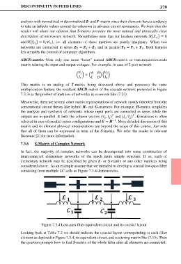
consisting from multiple LC-sells as Figure 7.3.4 demonstrates.

Figure 7.3.4 Low-pass filter equivalent circuit and its coaxial layout
Looking back at Table 7.2 we should indicate the coaxial layout corresponding to each filter
element as depicted in Figure 7.3.4, its equivalent circuit, and scattering matrix like (7.15). Then
the question prompts how to find S-matrix of the whole filter after all elements are connected.