Page 400 - Maxwell House

380 Chapter 7

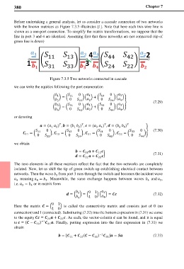
Before undertaking a general analysis, let us consider a cascade connection of two networks
with the known matrices as Figure 7.3.5 illustrates [1]. Note that here each two-wire line is
shown as a one-port connection. To simplify the matrix transformations, we suppose that the
line in port 3 and 4 are identical. Assuming first that these networks are not connected (tip of
green line is down)

Figure 7.3.5 Two networks connected in cascade

we can write the equities following the port enumeration

0 1 0 3
1
� � = � 11 � � � + � 13 � � �
0 2 0 4
2 22 24 � (7.29)
0 1 0 3
3
� � = � 31 � � � + � 33 � � �
4 0 42 2 0 44 4
or denoting

= ( ) , = ( ) , = ( ) , = ( )
1 2 1 2 3 4 3 4
0 0 0 0 � (7.30)
11 = � 11 � , 12 = � 13 � , 21 = � 31 � , 22 = � 33 �
0 22 0 24 0 42 0 44
we obtain
= +
11 12 � (7.31)
= +
21
22
The zero elements in all these matrices reflect the fact that the two networks are completely
isolated. Now, let us shift the tip of green switch up establishing electrical contact between
networks. Then the wave from port 3 runs through the switch and becomes the incident wave
3
meaning = . Meanwhile, the same exchange happens between waves and ,
3
4
4
3
4
i.e. = or in matrix form
3 4
3 0 1 3
= � � = � � � � = (7.32)
1 0 4
4
0 1
Here the matrix = � � is called the connectivity matrix and consists just of 0 (no
1 0
connection) and 1 (connected). Substituting (7.32) into the bottom expression in (7.31) we come
to the equity = + . As such, the vector-column can be found, and it is equal
21
22
to = ( − ) . Finally, putting expression into the first expression in (7.31) we
−1
22
21
obtain
−1
= [ 11 + ( − ) ] = (7.33)
12
22
21