Page 478 - Maxwell House

458 Chapter 9

9.2 GRID AND CLOUD COMPUTING

9.2.1 Introduction
We assume that the reader became compatible with the basic idea of primary numerical methods
that can help monitor and understand more complicated ways with relative ease. Furthermore,
we are not going to discuss any details of the frequency-domain variants. They follow the same
discretization path and often slightly more simple due to the given time dependence exp ().
As a result, all time-domain operations and transformations disappear thereby reducing the
problem dimension. In such context, the simulation in frequency domain requires commonly
less training and more efficient, depending on the research area and computer resources on
hand. Our current objective is to show how to accelerate the numerical simulations. That will
go mainly about FDTD method that naturally lends itself to parallelization on High-
Performance Computers (HPC).

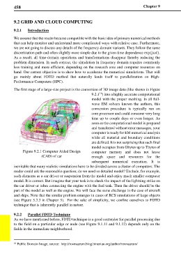
The first stage of a large-size project is the conversion of 3D image data (like shown in Figure
16
9.2.1 ) into a highly accurate computational
model with the proper meshing. In all full-
wave EM solvers known the authors, this
conversion procedure is typically run on
core processor and could consume very long
time up to couple days or even longer. As
soon as the computational model is prepared
and transferred without error messages, your
computer is ready for EM numerical analysis
while all material and boundary conditions
are defined. It is not surprising that such final
model occupies from Gbytes up to Tbytes of
Figure 9.2.1 Computer Aided Design computer memory and does not leave
(CAD) of car enough space and resources for the
subsequent numerical execution. It is
inevitable that many realistic simulations have to be divided across a cluster of computers. The
reader could ask the reasonable question; do we need so detailed model? Exclude, for example,
such elements as a car driver or suspension from the model and enjoy much smaller computer
model. It is correct. But imagine that your task is to check the impact of the lightning strike on
the car driver or tubes connecting the engine with the fuel tank. Then the driver should be the
part of the model as well as the engine. We will face the same challenge in the case of aircraft
and ships. Note that the similar problem emerges in cases of RCS simulations of large objects
(see Figure 5.3.3 in Chapter 5). For the sake of simplicity, we confine ourselves to FDTD
technique that is inherently parallel in nature.

9.2.2 Parallel FDTD Technique
As we have mentioned before, FDTD technique is a good contender for parallel processing due
to the field on a particular edge or node (see Figure 9.1.11 and 9.1.12) depends only on the
fields in the immediate neighborhood.

16 Public Domain Image, source: http://rosmaarum.blog.binusian.org/author/rosmaarum/