Page 474 - Maxwell House

454 Chapter 9

more flexible diminishing this effect and shorting solution time but complicating the algorithm
realization.
• Standard FDTD algorithm cannot support the metamaterials with negative values of relative
permittivity or permeability. As
soon as these parameters become
less than unity, the algorithm might
not be stable.
• Cumulative errors for long
duration and propagation distances.
• Hard to model materials with
frequency dependent (dispersive)
properties.
• The accuracy is around one order
of magnitude worse than MoM of
the same shape.
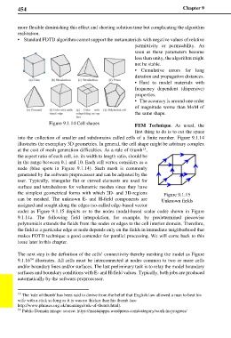
Figure 9.1.14 Cell shapes FEM Technique. As usual, the
first thing to do is to cut the space
into the collection of smaller and subdomains called cells of a finite number. Figure 9.1.14
illustrates the exemplary 3D geometries. In general, the cell shape might be arbitrary complex
13
at the cost of mesh generation difficulties. As a rule of thumb ,
the aspect ratio of each cell, i.e. its width to length ratio, should be
in the range between 0.1 and 10. Each cell vertex considers as a
node (blue spots in Figure 9.1.14). Such mesh is commonly
generated by the software preprocessor and can be adjusted by the
user. Typically, triangular flat or curved elements are used for
surface and tetrahedrons for volumetric meshes since they have
the simplest geometrical forms with which 2D- and 3D-regions Figure 9.1.15
can be meshed. The unknown E- and H-field components are Unknown fields
assigned and sought along the edges (so-called edge-based vector
code) as Figure 9.1.15 depicts or to the nodes (nodal-based scalar code) shown in Figure
9.1.14a. The following field interpolation, for example, by predetermined piecewise
polynomials extends the fields from the nodes or edges to the cell interior domain. Therefore,
the field at a particular edge or node depends only on the fields in immediate neighborhood that
makes FDTD technique a good contender for parallel processing. We will come back to this
issue later in this chapter.

The next step is the definition of the cells’ connectivity thereby meshing the model as Figure
9.1.16 illustrates. All cells must be interconnected at nodes common to two or more cells
14
and/or boundary lines and/or surfaces. The last preliminary task is to relay the model boundary
surfaces and boundary conditions with E- and H-field values. Typically, both jobs are produced
automatically by the software preprocessor.

13 The 'rule of thumb' has been said to derive from the belief that English law allowed a man to beat his
wife with a stick so long as it is was no thicker than his thumb (see
http://www.phrases.org.uk/meanings/rule-of-thumb.html).
14 Public Domain image: source: https://mastajappa.wordpress.com/category/work-in-progress/