Page 469 - Maxwell House

APPROACH TO NUMERICAL SOLUTION OF EM PROBLEMS 449

ℳ�(, )� = ∑ ∞ ∑ ∞ ℳ( () ()) = (, ) (9.2)
=1

=

Here ℳ�(, )� is the entire set of integral and/or differential operations required by
Maxwell’s equations and (, ) is the given continuous function describing the spatial and
temporal distribution of EM field sources. The last step is to solve (9.2) minimizing, for
example, the residual
2
min( | ∑ ∑ ℳ( () ()) − (, )| ) (9.3)

=
=1

,
Note that the sequences are truncated reflecting the fact that computers cannot deal with infinite
series. Generally speaking, the expression (9.3) is equivalent to the search of the stable solution
by minimizing the energy stored in the system. How to do it effectively is typically the
proprietary information (trade secret) of the company developing a particular CEM product and
result of extensive and in-depth mathematical research. The critical issue here is the choice of
suitable basis functions solving the problem (9.3).
The core strengths of MoM technique are:
• Physically transparent and relatively simple to implement.
• Ability to simulate the radiation problems with open boundaries naturally (see Section 3.3.1
in Chapter 3) by including into algorithm the basis functions (like Green’s functions (4.34) in
Chapter 4) satisfying the radiation condition (3.72) thereby possessing the correct far-field
behavior.
• Efficient treatment of perfectly or highly conducting objects’ faces requiring the surface
meshing only that significantly simplify the discretization procedure, reduce computer memory
storage and simulation time. That is probably the best tool for large antenna design or metal
scatterers like aircraft as soon as their metal surfaces can be treated as wire grid.
• Working well for small as well as vast structures (relative to wavelength).

The primary drawbacks of MoM technique are:
• Relatively poor handling dielectric objects where EM waves penetrate their surface.
• Commonly, it leads to systems of linear equations having dense matrices of × , where
is the total number of unknown coefficient in (9.3). If so, the required computer storage is
proportional to . The computer execution time to invert such matrix, i.e. find a solution,
2
varies between to depending on matrix structure and chosen inversion algorithm.
2
3
• Error analysis is not straightforward.
Any further discussion of such deep and arcane
mathematical subjects will lead us too far away
from this book contents. So we refer the reader to
the specialized literature [5, 6].

We know (see Table 1.7 in Chapter 1) that
Maxwell’s equations include the time derivative
of B-fields depending on the curl of E-fields and
H-field is proportional to B-field, D-field depends
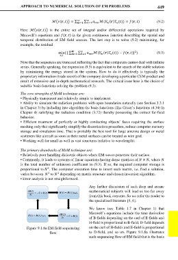
Figure 9.1.8a EM field sequencing on the curl of H-fields and E-field is proportional
flow to D-field, and so on. Figure 9.1.8a illustrates
such sequencing flow of EM field that is the basis