Page 467 - Maxwell House

APPROACH TO NUMERICAL SOLUTION OF EM PROBLEMS 447

9.1.2 Basic Numerical Methods in Computational Electrodynamics (CEM)
Up to this point, we did not touch the theme how to choose the “best-fit” for your particular
task EM modeling software or manage the currently available in your organization. As of the
date of the publication, we found, probably,
more than hundred different tools .
8
Nevertheless, the single “best-fit” method for
all circumstances is a recurring and lucid
dream despite the fact that new software
variations are continuously developed. The
heart and brain of any EM computational code
are the evaluated in this code digital image of
Maxwell’s equations and the path to their
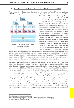
solution. Figure 9.1.6 illustrates the simple
diagram sorting different approaches [2]. The
abbreviations of Figure 9.1.6 are: VIE = Vector
Integral Equations, VPDE = Vector Partial
Differential Equations, VVE = Vector Wave
Equations, MoM = Method of Moments,
Figure 9.1.6 Classification of basic FDTD = Finite-Difference Time-Domain,
numerical methods FEM = Finite Element Method, and FDFD =
Finite-Difference Frequency-Domain.
Probably, the most challenging and time-consuming mission indicated in this diagram is the
development of a professional and bug-free computer program with user-friendly interface. A
slightly different but more complete diagram is shown in Figure 9.1.7 . For more details, the
9
reader can turn to [15]. We advise considering any of such diagram as idealized and incomplete
because many of techniques are hybridized and interconnected with each other.
The subject of CEM algorithm is too broad to be covered in several pages or even a single
chapter, and thus only a synoptic view, straightforward and as compact as possible is given
below. Evidently, the time and frequency domain Maxwell’s equations convey the exact same
information about EM fields. This fact is illustrated by Fourier transform (1.88) from Chapter
1 interconnecting these two forms of the solution. Typically, the time domain algorithms are
realized assuming that the field sources inject energy for short time measured in microseconds
or even shorter. If so, this solution is the set of pulses propagating in the space. Applying Fourier
transform to each of these pulses, we can extract the field intensities at the frequencies
belonging to the pulse spectrum. Since the spectrum of short rectangular or Gaussian pulse
comprises, at least theoretically, an infinite number of components, the obtained solution
reveals information on many frequencies at the same time. Note that the information about the
transient far-fields becomes increasingly important in ultra-wideband (UWB) applications. For
example, in multiport communication or radar systems, every port can be excited individually
with a different time varying signal, and the composite fields are monitored in the time domain.

8 http://www.cvel.clemson.edu/modeling/
9 Public Domain Image reprinted with Dr. Li Er-Ping’s permission, source [15]:
http://web.mst.edu/~jfan/slides/li2.pdf