Page 470 - Maxwell House

450 Chapter 9

of Yee cells discretization considered below. FDTD method [4] is the direct solution of
Maxwell’s equations, conceptually simple, and
probably the most powerful and versatile
numerical method. We know (see Table 1.7 in
Chapter 1) that Maxwell’s equations include the
time derivative of B-fields depending on the curl
of E-fields and H-field is proportional to B-field,
D-field depends on the curl of H-fields and E-field
is proportional to D-field, and so on. Figure 9.1.8a
illustrates such sequencing flow of EM field that
is the basis of Yee cells discretization considered
Figure 9.1.8b Central difference below.

The curls, in turn, are a combination of the first order spatial coordinate derivatives. If so, each
of spatial or time derivatives can be replaced, as a calculus course tells us, with some level
accuracy by finite (for example, central) differences. Figure 9.1.8b demonstrates the exemplary
procedure for 1D function. If the value of ∆ = +1 − −1 is small enough and the
′ ∆ 2
function () is smooth, then ( ) ≅ + (∆ ). Here the numerator ∆ = +1 − −1

∆
is referred to as a central difference. The “big-
Oh” represents all the terms that are not explicitly
shown and the value in parentheses, i.e. ∆ ,
2
indicates the lowest order of ∆ in these hidden
terms. Since the lowest power of ∆ being
ignored is second order, the presented central
difference is said to have second-order accuracy
or second-order behavior. More accurate
approximations can be performed treating the
function y(x) like a polynomial of second, third

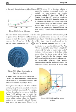
Figure 9.1.9 Sphere discretization in
Cartesian coordinates
or higher order in the neighborhood of .

Clearly, the above-mentioned approximation
can be extended to 3D regions discretized into
cells of smaller sizes (typically < /10).

Although theoretically, the cell shape could be
arbitrary, the preferable coordinate system is
Cartesian that leads to cubic cells. For example,
a sphere discretized in this manner looks like
Figure 9.1.9 pictures. As a result, the
computational image does not perfectly imitate
curved object surface where the boundary Figure 9.1.10 Cell touching sphere
conditions are commonly defined. Thereby surface
some errors are unavoidable. Figure 9.1.10