Page 471 - Maxwell House

APPROACH TO NUMERICAL SOLUTION OF EM PROBLEMS 451

demonstrates this phenomenon: E- and H-fields positioned on the cell surface are close but do
not belong to the surface of a sphere.
The most popular discretization lattice and based on it numerical technique was proposed by
K. S. Yee in 1966 and carries his name. Yee cells discretize E- and H-field into components as
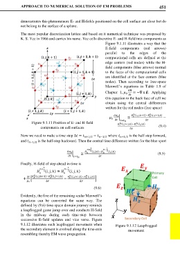
Figure 9.1.11 illustrates a way that the
E-field components (red arrows)
parallel to the edges of the
computational cells are defined at the
edge centers (red nodes) while the H-
field components (blue arrows) normal
to the faces of the computational cells
are identified at the face centers (blue
nodes). Then according to free-space
Maxwell’s equations in Table 1.9 of

Chapter 1, 0 = − x . Applying
this equation to the back face of cell we
obtain using the central differences
written for the red nodes (free space)

(,,+1)− (,+1,)

0 � ≅ −
Figure 9.1.11 Position of E- and H-field = ∆

(,+1,)− (,,)
components on cell surfaces ∆ (9.4)
Now we need to make a time step ∆ = +1/2 − −1/2 where +1/2 is the half-step forward,
and is the half-step backward. Then the central time difference written for the blue sport
−1/2
1 1
+ −
2 (,,)− 2 (,,)
(9.5)
� ≅
∆
=
Finally, H-field of step ahead in time is
1 1
+ −
2 (, , ) ≅ 2 (, , ) Primary

∆ (,,+1)− (,+1,) (,+1,)− (,,) Cell
+ � − �
0 ∆ ∆
(9.6)
Evidently, the five of the remaining scalar Maxwell’s
equations can be converted the same way. The
defined by (9.6) time-space domain journey reminds
a leapfrogged game jump over and conducts H-field
in the midway during each time-step between
successive E-field updates and vice versa. Figure Secondary Cell
9.1.12 illustrates such leapfrogged movement when Figure 9.1.12 Leapfrogged
the secondary element is evolved along the time-axis movement
resembling thereby EM wave propagation.