Page 472 - Maxwell House

452 Chapter 9

A few words are how to choose the shape of a pulse waveform of the embedded source with
the broad spectrum of frequencies to support the postprocessing Fourier transform. Evidently,
it should be short and, at least theoretically, comprise an infinite number of components. Then
the obtained solution reveals information on many frequencies at the same time. Commonly
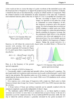
used untainted Gaussian pulses (blue line in Figure 9.1.13a) is acceptable but sometimes not
the best. According to Figure 9.1.13b (blue
image), the spectrum of this pulse has a large
dc component (or carrier frequency). In fact,
this frequency component carries the greatest
energy. It is hard to imagine that one would use
FDTD technique to model such static fields.
The first thought is to reduce the pulse duration
thereby extending its frequency coverage. But
the punishment might follow as the potential
Figure 9.1.13a Gaussian (blue) and conversion slow down and appearance of not
Ricker (green) pulse envelope physical artifacts. If so, more suitable spectrum
should be shifted to the frequencies of highest
interest. Taking the second derivative of a
Gaussian, we will obtain the symmetrically shaped pulse (so-called Ricker or Mexican hat
wavelet) with envelope () and power
spectrum magnitude () pictured in Figure
9.1.13a and b (green lines), respectively, and
described as

2
2
() = (1 − 2[ ] )exp(−[ ] )
0
0
2 2 �
2
() = � � exp �− � � �
√ 0 0 0
(9.7)
Here, is the frequency of the greatest Figure 9.1.13b Gaussian (blue) and Ricker
0
spectral component. (green) spectrum envelope
The core strengths of FDTD technique are:
• Conceptually simple to understand and naturally follows from Maxwell’s equations. The
developed model and simulation result correctness can be easily verified through E- and H-field
step-by-step animation. The algorithm makes use of the memory in a simple sequential order
simplifying the discretization process. As a result, CEM even of 3D simulation can be written
in a matter of minutes.
• Give response over a wide range of frequencies with a single run. Much easier to obtain
frequency domain data through Fast Fourier Transform (FFT) from FDTD transient data than
the converse.
• A broad variety of linear and nonlinear materials can be naturally modeled while the
numerical complexity is practically independent of objects’ shape.
• The traditional explicit FDTD method is matrix-free, i.e. no linear algebra or matrix
inversions are involved. As such, there is no inherent limit, at least in theory, to the size of a
simulation except the computation time. To keep traditional FDTD procedure stable, the time
step at which the solution advances is generally restrained by the spatial increment =