Page 468 - Maxwell House

448 Chapter 9

Such large-scale simulations are usually performed on distributed memory computing clusters
and shared memory
multiprocessors [3].

On the other hand, the
frequency domain
simulation must be repeated
as many times as required by
the problem to be solved or
in parallel on several
computers connected to the
grid. Nevertheless, it does
not mean that the time-
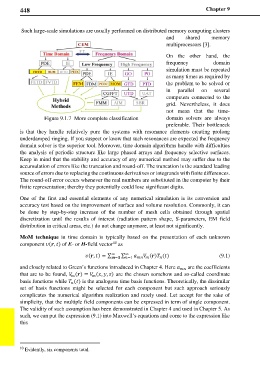
Figure 9.1.7 More complete classification domain solvers are always
preferable. Their bottleneck
is that they handle relatively pure the systems with resonance elements creating prolong
underdamped ringing. If you suspect or know that such resonances are expected the frequency
domain solver is the superior tool. Moreover, time domain algorithms handle with difficulties
the analysis of periodic structure like large phased arrays and frequency selective surfaces.
Keep in mind that the stability and accuracy of any numerical method may suffer due to the
accumulation of errors like the truncation and round-off. The truncation is the standard leading
source of errors due to replacing the continuous derivatives or integrands with finite differences.
The round-off error occurs whenever the real numbers are substituted in the computer by their
finite representation; thereby they potentially could lose significant digits.

One of the first and essential elements of any numerical simulation is its conversion and
accuracy test based on the improvement of surface and volume resolution. Commonly, it can
be done by step-by-step increase of the number of mesh cells obtained through spatial
discretization until the results of interest (radiation pattern shape, S-parameters, EM field
distribution in critical areas, etc.) do not change anymore, at least not significantly.
MoM technique in time domain is typically based on the presentation of each unknown
10
component (, ) of E- or H-field vector as
(, ) = ∑ ∞ ∑ ∞ () () (9.1)
= =1
and closely related to Green’s functions introduced in Chapter 4. Here are the coefficients
that are to be found, () = (, , ) are the chosen somehow and so-called coordinate

basis functions while () is the analogous time basis functions. Theoretically, the dissimilar

set of basis functions might be selected for each component but such approach seriously
complicates the numerical algorithm realization and rarely used. Let accept for the sake of
simplicity, that the multiple field components can be expressed in term of single component.
The validity of such assumption has been demonstrated in Chapter 4 and used in Chapter 5. As
such, we can put the expression (9.1) into Maxwell’s equations and come to the expression like
this

10 Evidently, six components total.