Page 465 - Maxwell House

APPROACH TO NUMERICAL SOLUTION OF EM PROBLEMS 445

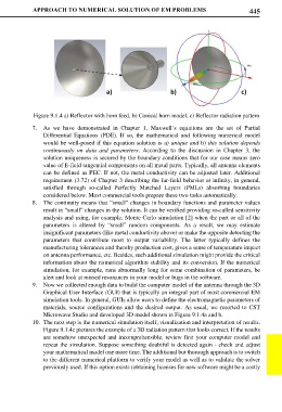
Figure 9.1.4 a) Reflector with horn feed, b) Conical horn model, c) Reflector radiation pattern

7. As we have demonstrated in Chapter 1, Maxwell’s equations are the set of Partial
Differential Equations (PDE). If so, the mathematical and following numerical model
would be well-posed if this equation solution is a) unique and b) this solution depends
continuously on data and parameters. According to the discussion in Chapter 3, the
solution uniqueness is secured by the boundary conditions that for our case means zero
value of E-field tangential components on all metal parts. Typically, all antenna elements
can be defined as PEC. If not, the metal conductivity can be adjusted later. Additional
requirement (3.72) of Chapter 3 describing the far-field behavior at infinity, in general,
satisfied through so-called Perfectly Matched Layers (PMLs) absorbing boundaries
considered below. Most commercial tools prepare these two tasks automatically.
8. The continuity means that “small” changes in boundary functions and parameter values
result in “small” changes in the solution. It can be verified providing so-called sensitivity
analysis and using, for example, Monte Carlo simulation [2] when the part or all of the
parameters is altered by “small” random components. As a result, we may estimate
insignificant parameters (like metal conductivity above) or make the opposite detecting the
parameters that contribute most to output variability. The latter typically defines the
manufacturing tolerances and thereby production cost, gives a sense of temperature impact
on antenna performance, etc. Besides, such additional simulation might provide the critical
information about the numerical algorithm stability and its conversion. If the numerical
simulation, for example, runs abnormally long for some combination of parameters, be
alert and look at missed resonances in your model or bugs in the software.
9. Now we collected enough data to build the computer model of the antenna through the 3D
Graphical User Interface (GUI) that is typically an integral part of most commercial EM
simulation tools. In general, GUIs allow users to define the electromagnetic parameters of
materials, source configurations and the desired output. As usual, we resorted to CST
Microwave Studio and developed 3D model shown in Figure 9.1.4a and b.
10. The next step is the numerical simulation itself, visualization and interpretation of results.
Figure 9.1.4c pictures the example of a 3D radiation pattern that looks correct. If the results
are somehow unexpected and incomprehensible, review first your computer model and
repeat the simulation. Suppose something doubtful is detected again - check and adjust
your mathematical model one more time. The additional but thorough approach is to switch
to the different numerical platform to verify your model as well as to validate the solver
previously used. If this option exists (obtaining licenses for new software might be a costly