Page 475 - Maxwell House

APPROACH TO NUMERICAL SOLUTION OF EM PROBLEMS 455

To form a linear system of equations, the governing Maxwell’s equations and associated
boundary conditions are converted to the integrodifferential form using either a variational
method like (9.3), i.e. minimizing the accumulated by the system EM energy, or approximating
the source distribution and desired solution by the linear combination of basis functions. The
15
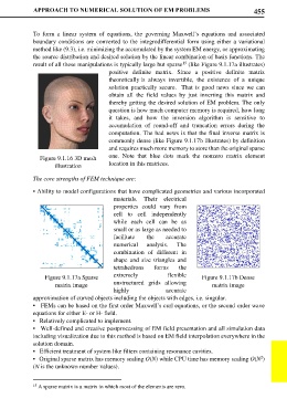
result of all these manipulations is typically large but sparse (like Figure 9.1.17a illustrates)
positive definite matrix. Since a positive definite matrix
theoretically is always invertible, the existence of a unique
solution practically secure. That is good news since we can
obtain all the field values by just inverting this matrix and
thereby getting the desired solution of EM problem. The only
question is how much computer memory is required, how long
it takes, and how the inversion algorithm is sensitive to
accumulation of round-off and truncation errors during the
computation. The bad news is that the final inverse matrix is
commonly dense (like Figure 9.1.17b illustrates) by definition
and requires much more memory to store than the original sparse
Figure 9.1.16 3D mesh one. Note that blue dots mark the nonzero matrix element
illustration location in this matrices.

The core strengths of FEM technique are:
• Ability to model configurations that have complicated geometries and various incorporated
materials. Their electrical
properties could vary from
cell to cell independently
while each cell can be as
small or as large as needed to
facilitate the accurate
numerical analysis. The
combination of different in
shape and size triangles and
tetrahedrons forms the
Figure 9.1.17a Sparse extremely flexible Figure 9.1.17b Dense
matrix image unstructured grids allowing matrix image
highly accurate
approximation of curved objects including the objects with edges, i.e. singular.
• FEMs can be based on the first order Maxwell’s curl equations, or the second order wave
equations for either E- or H- field.
• Relatively complicated to implement.
• Well-defined and creative postprocessing of EM field presentation and all simulation data
including visualization due to this method is based on EM field interpolation everywhere in the
solution domain.
• Efficient treatment of system like filters containing resonance cavities.
2
• Original sparse matrix has memory scaling O(N) while CPU time has memory scaling O(N )
(N is the unknown number values).

15 A sparse matrix is a matrix in which most of the elements are zero.