Page 485 - Maxwell House

APPENDIX 465

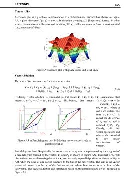
Contour Plot

A contour plot is a graphical representation of a 3-dimensional surface like shown in Figure
A4. It plots the curve (, ) = . in the plane xy using a 2-dimensional format. In other
words, these curves are the slices of function (, ), called contours or level or equipotential
(i.e., isopotential) lines.

Figure A4 Surface plot with plane slices and level lines
Vector Addition

The sum of two vectors is defined as a new vector

= + = � + + � + � + + � (A.4)
0 2
0 1
0 1
0 1
2
1
0 2
0 2
= ( + ) + ( + ) + ( + )
0 1 2 0 1 2 0 1 2
Evidently, vector addition is commutative, that means + = + , associative, that
1
1
2
2
means + ( + ) = ( + ) + , distributive, that means ( + ) = +
2
3
1
2
1
3
and ( + ) =
2
1
+ , where a
1
2
and b are scalars. The
sum +(− ) is
2
1
called the difference
of and and is
1
2
denoted by − .
1
2
Clearly, all this
vector operations and
rules can be extended
to any linear
Figure A5 a) Parallelogram law, b) Moving vector successively to combination of
parallel position
vectors.
Parallelogram Law. Graphically the vector sum + can be represented by the diagonal of
2
1
a parallelogram formed by the vectors and as shown in Figure A5a. Eventually, we will
1
2
obtain the same result moving the vector successively to parallel position as shown in Figure
2
A5b when the head of one vector connects to the tail of the next vector. The sum is the vector
whose tail connects to the tail of the first vector, and whose head connects to the head of the
last vector. The vectors addition and difference based on the parallelogram law is illustrated in
Figure A6.